Using Oracle Data Miner 4.0 with Big Data Lite 4.0
Overview
- Predict individual behavior, for example, the customers likely to respond to a promotional offer or the customers likely to buy a specific product (Classification)
- Find profiles of targeted people or items (Classification using Decision Trees)
- Find natural segments or clusters (Clustering)
- Identify factors more associated with a target attribute (Attribute Importance)
- Find co-occurring events or purchases (Associations, sometimes known as Market Basket Analysis)
- Find fraudulent or rare events (Anomaly Detection)
- Problem Definition in Terms of Data Mining and Business Goals
- Data Acquisition and Preparation
- Building and Evaluation of Models
- Deployment
Purpose
This tutorial covers the use of Oracle Data Miner 4.0 to perform data mining activities on the Big Data Lite 4.0 VM, which runs Oracle Database 12c Release 1. Oracle Data Miner 4.0 is included as an extension of Oracle SQL Developer, version 4.0, which is also included on the VM.
In this lesson, you learn how to use Data Miner to create a classification model in order to predict the company's likely best customers.
Time to Complete
Approximately 30 mins.
Introduction
Data mining is the process of extracting useful information from masses of data by extracting patterns and trends from the data. Data mining can be used to solve many kinds of business problems, including:
The phases of solving a business problem using Oracle Data Mining are as follows:
Problem Definition and Business Goals
When performing data mining, the business problem must be well-defined and stated in terms of data mining functionality. For example, retail businesses, telephone companies, financial institutions, and other types of enterprises are interested in customer “churn” – that is, the act of a previously loyal customer in switching to a rival vendor. The statement “I want to use data mining to solve my churn problem” is much too vague. From a business point of view, the reality is that it is much more difficult and costly to try to win a defected customer back than to prevent a disaffected customer from leaving; furthermore, you may not be interested in retaining a low-value customer. Thus, from a data mining point of view, the problem is to predict which customers are likely to churn with high probability, and also to predict which of those are potentially high-value customers.
Data Acquisition and Preparation
A general rule of thumb in data mining is to gather as much information as possible about each individual, then let the data mining operations indicate any filtering of the data that might be beneficial. In particular, you should not eliminate some attribute because you think that it might not be important – let ODM’s algorithms make that decision. Moreover, since the goal is to build a profile of behavior that can be applied to any individual, you should eliminate specific identifiers such as name, street address, telephone number, etc. (however, attributes that indicate a general location without identifying a specific individual, such as Postal Code, may be helpful.) It is generally agreed that the data gathering and preparation phase consumes more than 50% of the time and effort of a data mining project.
Building and Evaluation of Models
The Workflow creation process of Oracle Data Miner automates many of the difficult tasks during the building and testing of models. It’s difficult to know in advance which algorithms will best solve the business problem, so normally several models are created and tested. No model is perfect, and the search for the best predictive model is not necessarily a question of determining the model with the highest accuracy, but rather a question of determining the types of errors that are tolerable in view of the business goals.
Deployment
Oracle Data Mining produces actionable results, but the results are not useful unless they can be placed into the correct hands quickly. The Oracle Data Miner user interface provides several options for publishing the results.
Scenario
This lesson focuses on a business problem that can be solved by applying a Classification model. In our scenario, the Electrionics R Us company wants to identify customers who are most likely to be the best customers in terms of sales.
Note: For the purposes of this tutorial, the "Data and Acquisition" phase has already been completed, and the sample data set contains all required data fields. Therefore, this lesson focuses primarliy on the "Building and Evaluation of Models" phase.
Software Requirements
This tutorial requires Oracle BIg Data Lite Virtual Machine (VM). You can download the VM from the Big Data Lite page on OTN.
Prerequisites
None
Create a Data Miner Project
- If the Data Miner tab is not open, select Tools > Data Miner > Make Visible from the SQL Developer menubar.
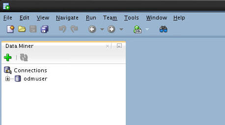
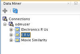
- As shown above, the data miner user (odmuser) has been created and a SQL Developer connection has been established for this user.
- There are two Data Miner projects that have already been created for this user.
To begin, click the SQL Developer program icon at the menu bar.
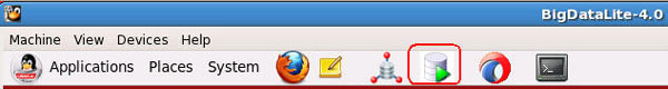
Result: Oracle SQL Developer opens.
Before you create a Data Miner Project and build a Data Miner workflow, it is helpful to organize the Data Miner interface components within SQL Developer to provide simplified access to Data Miner features.
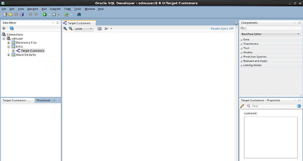
Therefore, close all of the SQL Developer interace elements (which may include the Start Page tab, the Connections tab, the Reports tab, and others). Leave only the Data Miner tab open, like this:
Notes:
Next, you will create new Data Miner Project.
Create a Data Miner Project
Before you begin working on a Data Miner Workflow, you must create a Data Miner Project, which serves as a container for one or more Workflows.
To create a Data Miner Project, perform the following steps:
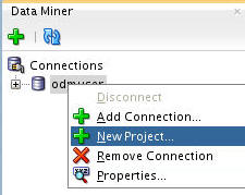
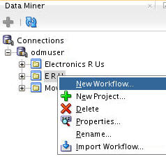
In the Data Miner tab, right-click odmuser and select New Project, as shown here:
In the Create Project window, enter the name E R U and then click OK.
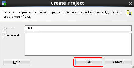
Note: You may optionally enter a comment that describes the intentions for this project. This description can be modified at any time.
Result: The new project appears below odmuser connection node.
Build a Data Miner Workflow
- Provides directions for the Data Mining server. For example, the workflow says "Build a model with these characteristics." The model is built by the data mining server with the results returned to the workflow.
- Enables you to interactively build, analyze, and test a data mining process within a graphical environment.
- May be used to test and analyze only one cycle within a particular phase of a larger process, or it may encapsulate all phases of a process designed to solve a particular business problem.
- Each element in the process is represented by a graphical icon called a node.
- Each node has a specific purpose, contains specific instructions, and may be modified individually in numerous ways.
- When linked together, workflow nodes construct the modeling process by which your particular data mining problem is solved.
- Identify and examine source data from two tables
- Build and compare several Classification models
- Select and run the models that produce the most actionable results
- In the middle of the SQL Developer window, an empty workflow tabbed window opens with the name that you specified.
- On the upper right-hand side of the interface, the Components tab of the Workflow Editor appears.
- On the lower right-hand side of the interface, the Properties tab appears.
- In addition, two other Oracle Data Miner interface elements may be opened on the lower left-hand side of the interface:
- The Structure tab, with the name of the workfolw
- The Thumbnail tab
- Workspace node names and model names are generated automatically by Oracle Data Miner. In this example, the name "Data Source" is generated. You may not get exactly the same node and model names as shown in this lesson. You can change the name of any workspace node or model using the Property Inspector.
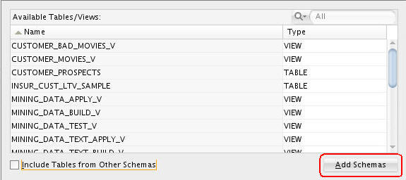
- Only those tables and views that are in the user's schema are displayed by default. Next, you add objects to the list from other schemas to which odmuser has been given access.
- Right-click the data source node and select Connect from the pop-up menu.
- Drag the pointer to the Join node and click again.
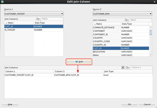
- Select CUSTOMER_TARGET as Source 1, andCUSTOMER_RFM as Source 2.
- Select the CUST_ID column from both sources.
- Then, click the Add button to define the Join Columns.
- Deselect the Automatic Settings option (top left side of Columns tab).
- Scroll down to the bottom of the Output Data Columns list, and select the USERNAME column from the CUSTOMER_RFM node.
- Click the Remove tool (red "x" icon).
- Click Yes in the Warning window.
- Recall that a yellow Information (!) icon in the border around any node indicates that it is not complete.
- In this case, you must connect a data source to the Explore Data node to enable further exploration of the source data.
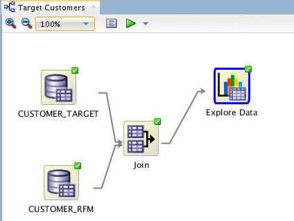
- Data Miner saves the workflow document, and displays status information at the top of the Workflow pane while processing the node.
- As each node is processed, a green gear icon displays in the node border.
- When the update is complete, the data source and explore data nodes show a green check mark in the borders, like this:
- Data Miner calculates a variety of statistics about each attribute in the data set, as it relates to the "Group By" attribute that you previously defined (IS_TARGET). Output columns include: a Histogram thumbnail, Data Type, Distinct Values, Distinct Percent, Mode, Average, Median, Min and Max value, Standard Deviation, and Variance.
- The display enables you to visualize and validate the data, and also to manually inspect the data for patterns or structure.
- A Filter Columns node may be used to specify additional instructions for Attribute Importance for the Target variable. The filter node will provide suggestions on which variables to include/exclude based on data quality filters, and the attribute importance of each input variable.
- This extra, optional step theoretically reduces “noisy” less relevant input variables.
- You can ignore the recommendations, implement the recommendations for all columns, or selectively choose to implement some of the recommendations.
- In this case, you will implement all recommendations accept for the CUST_ID column.
- As stated previously, a yellow exclamation mark on the border indicates that more information needs to be specified before the node is complete.
- In this case, two actions are required:
- A connection must be created between the Filter Columns node and the classification build node.
- Two attributes should be specified for the classification build process.
- Notice that a yellow "!" indicator is displayed next to the Target and Case ID fields. This means that an attribute must be selected for these items.
- The names for each model are automatically generated, and yours may differ slightly from those in this example.
- A Case ID is used to uniquely define each record. This helps with model repeatability and is consistent with good data mining practices.
- As stated previously, all four algorithms for Classification modeling are selected by default. They will be automatically run unless you specify otherwise.
- Whether or not to perform a test during the build process
- Which test results to generate
- How you want the test data managed
- When the node runs it builds and tests all of the models that are defined in the node.
- As before, a green gear icon appears on the node borders to indicate a server process is running, and the status is shown at the top of the workflow window.
- All four models have been succesfully built.
- The models all have the same target (IS_TARGET) but use different algorithms.
- The source data is automatically divided into test data and build data.
- The comparison results include five tabs: Performance, Performance Matrix, ROC, Lift, and Profit.
- The Performance tab provides numeric and graphical information for each model on Predictive Confidence, Average Accuracy, and Overall Accuracy.
- The Performance tab seems to indicate that the Decision Tree (DT) model is providing the highest predictive confidence, overall accuracy %, and average accuracy %. The other models show mixed results.
- The Lift tab provides a graphical presentation showing lift for each model, a red line for the random model, and a vertical blue line for threshold.
- Lift is a different type of model test. It is a measure of how “fast” the model finds the actual positive target values.
- The Lift viewer compares lift results for the given target value in each model.
- The Lift viewer displays Cumulative Positive Cases and Cumulative Lift.
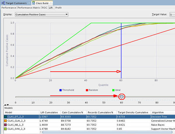
- As you move up the quantile range, the Lift Cumulative and Gain Cumulative % of the DT model separates a bit from the other models.
- As you move to the 60th quantile,the DT model shows a larger separation in terms of increased Lift and Gain.
- The Performance Matrix shows that the DT model has the highest Correct Predictions percentage. The other three models are close in the same metric.
- Your results may differ slightly, as each model build process takes a different sample.
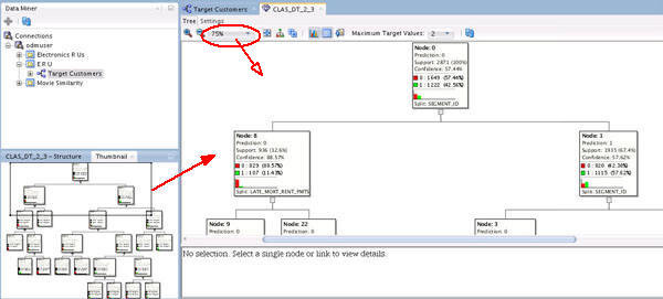
- The Thumbnail tab (located in the lower-left) provides a high level view of the entire tree. For example, the Thumbnail tab shows that this tree contains seven levels, although you view fewer of the nodes in the primary display window. By showing the entire tree, the Thumbnail tab also illustrates the particular branches that lead to the terminal node.
- You can move the viewer box around within the Thumbnail tab to dynamically locate your view in the primary window. You can also use the scroll bars in the primary display window to select a different location within the decision tree display.
- Finally, you can change the viewer percentage zoom in the primary display window to increase or decrease the size of viewable content.
- At each level within the decision tree, an IF/THEN statement that describes a rule is displayed. As each additional level is added to the tree, another condition is added to the IF/THEN statement.
- For each node in the tree, summary information about the particular node is shown in the box.
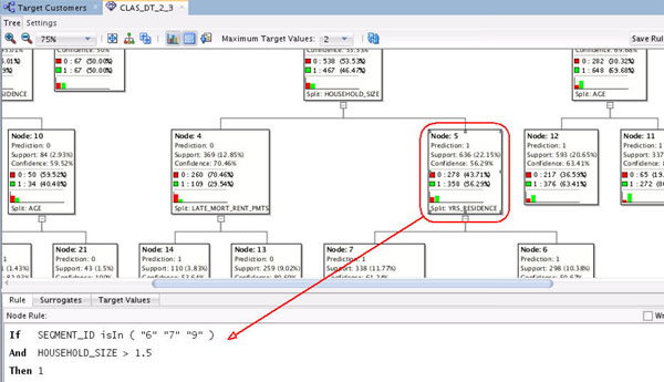
- In addition, the IF/THEN statement rule appears in the Rule tab, as shown below, when you select a particular node.
- At this level, we see that the first split is based on the SEGMENT_ID attribute, and the second split is based on the HOUSEHOLD_SIZE attribute.
- Node 5 indicates that if SEGMENT_ID IS 6, 7, OR 9, and HOUSEHOLD_SIZE is greater than 1.5, then there is a 56% chance that the customer is part of the target group.
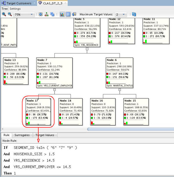
- At this node, the final splits are added for the YRS_RESIDENCE and YRS_CURRENT_EMPLOYER attributes.
- This node indicates that if YRS_RESIDENCE is greater than 14.5 and YRS_CURRENT_EMPLOYER is less than or equal to 14.5 years, then there is a 63.4% chance that the customer will be in the target group of best customers.
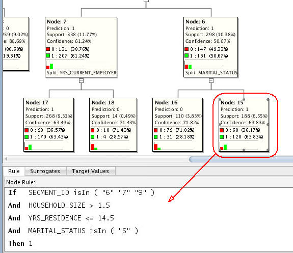
- At this node, the final splits are added for the YRS_RESIDENCE and MARITAL_STATUS attributes.
- This node indicates that if YRS_RESIDENCE is less than or equal to 14.5 and MARITAL_STATUS is "S" (Single), then there is a 63.8% chance that the customer will be in the target group of best customers.
- First, specify the desired model (or models) in the Class Build node.
- Second, add a new Data Source node to the workflow. (This node will serve as the "Apply" data.)
- Third, an Apply node to the workflow.
- Next, connect both the Class Build node and the new Data Source node to the Apply node.
- Finally, you run the Apply node to create predictive results from the model.
- The yellow exclamation mark disappears from the Apply Model node border once the second link is completed.
- This indicates that the node is ready to be run.
- The prediction: 1 or 0 (Yes or No)
- The probability of the prediction
- Select CUST_ID in the Available Attributes list.
- Move it to the Selected Attributes list by using the shuttle control.
- Then, click OK.
- The table contains four columns: three for the prediction data, and one for the customer ID.
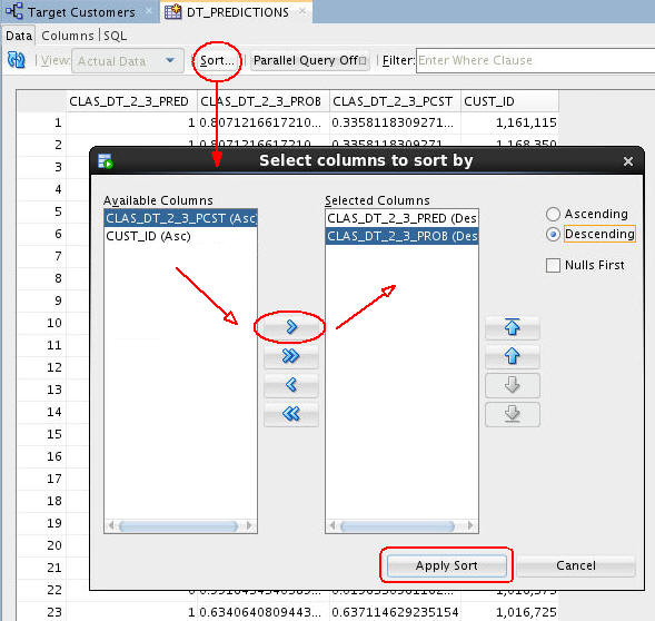
- You can sort the table results on any of the columns using the Sort button, as shown here.
- In this case, the table will be sorted using:
- First - the predicted outcome (CLAS_DT_2_3_PRED), in Descending order -- meaning that the prediction of "1" (Yes) for being classified as one of the best customers -- appears at the top of the table display.
- Second - prediction probability (CLAS_DT_2_3_PROB), in Descending order -- meaning that the highest prediction probabilities are at the top as well.
- Each time you run an Apply node, Oracle Data Miner takes a different sample of the data to display. With each Apply, both the data and the order in which it is displayed may change. Therefore, the sample in your table may be different from the sample shown here. This is particularly evident when only a small pool of data is available, which is the case in the schema for this lesson.
- You can also filter the table by entering a Where clause in the Filter box.
- The table contents can be displayed using any Oracle application or tools, such as Oracle Application Express, Oracle BI Answers, Oracle BI Dashboards, and so on.
A Data Miner Workflow is a collection of connected nodes that describe one or more data mining processes.
A workflow:
What Does a Data Miner Workflow Contain?
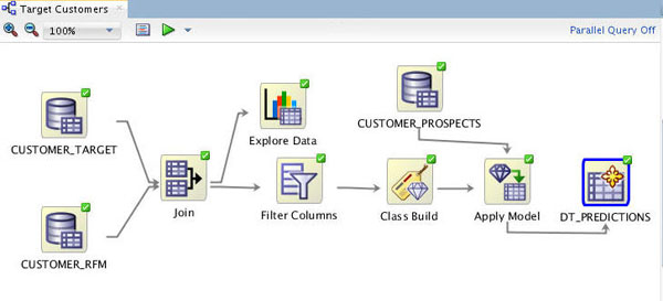
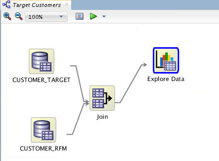
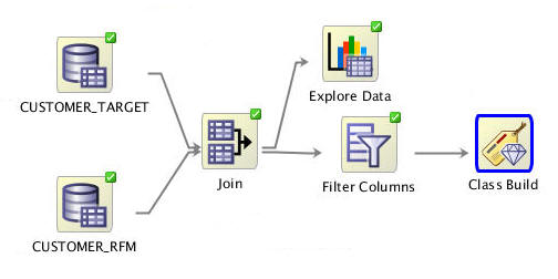
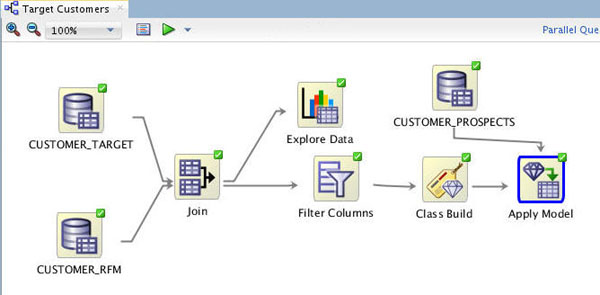
Visually, the workflow window serves as a canvas on which you build the graphical representation of a data mining process flow, like the one you are going to create, shown here:
Notes:
As you will learn, any node may be added to a workflow by simply dragging and dropping it onto the workflow area. Each node contains a set of default properties. You modify the properties as desired until you are ready to move onto the next step in the process.
Sample Data Mining Scenario
In this tutorial, you will create a data mining process that predicts those customers who should be targeted as one of the company's 'Best Customers'.
To accomplish this goal, you build a workflow that enables you to:
To create the workflow for this process, perform the following steps.
Create a Workflow, Add a Data Sources, and Join the Data
Right-click your project (E R U) and select New Workflow from the menu.
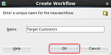
Result: The Create Workflow window appears.
In the Create Workflow window, enter Target Customers as the name and click OK.
Result:
As you will see later, you can open, close, resize, and move Data Miner tabbed panes around the SQL Developer window to suit your needs.
The first element of any workflow is the source data. Here, you add two Data Source nodes to the workflow that identify customer data.
A. In the Components tab, drill on the Data category. A group of six data nodes appear, as shown here:
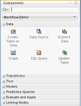
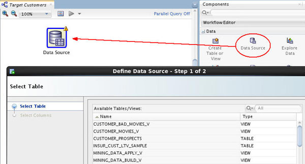
B. Drag and drop the Data Source node onto the Workflow pane.
Result: A Data Source node appears in the Workflow pane and the Define Data Source wizard opens.
Notes:
In Step 1 of the wizard:
A. Click the Add Schemas button below the Available Tables/Views box.
B. In the Edit Schema List dialog, select MOVIEDEMO in the Available list and move it to the Selected list, as shown here below. Then click OK.
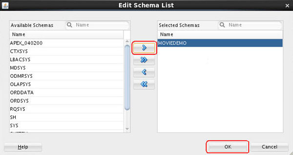
C. Next, select MOVIEDEMO.CUSTOMER_RFM from the Available Tables/Views list, as shown here:
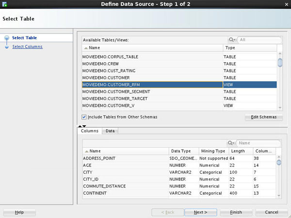
Note: You may use the two tabs in the bottom pane in the wizard to view the selected table or view. The Columns tab displays information about the table or view structure, and the Data tab shows a subset of data from the selected table or view.
D. Click Next to continue.
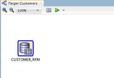
In Step 2 of the wizard, you may remove individual columns that you don't need in your data source. In our case, we'll keep all of the attributes that are defined in the view. At the bottom of the wizard window, click Finish.
Result: As shown below, the data source node name is updated with the selected table name, and the properties associated with the node are displayed in the Properties tab.
Next, add a second data source to the workflow using the same technique.
A. Drag and drop a Data Source node onto the workflow pane, just above the CUSTOMER.RFM node.
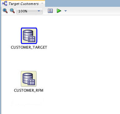
B. In Step 1 of the wizard, select MOVIEDEMO.CUSTOMER_TARGET from the list and click Finish.
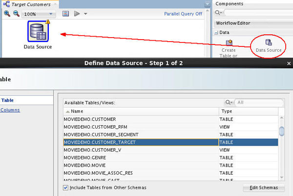
Result: As shown below, both data source nodes are displayed in the workflow pane.
Now, you join the tables to complete the data source definition.
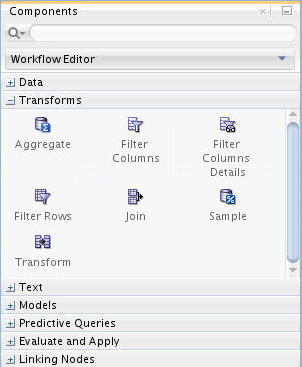
A. In the Components tab, collapse the Data category and drill on the Transforms category. A group of seven nodes appear, as shown here:
B. Drag and drop a Join node onto the workflow pane, as shown here:
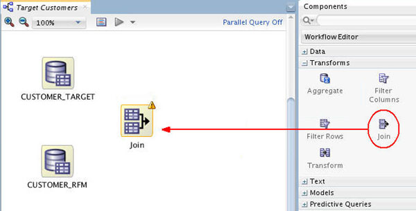
Note: A yellow Information (!) icon in the border around any node indicates that it is not complete. Therefore, at least one addition step is required before the node can be used.
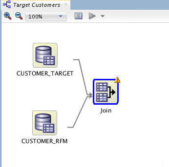
C. Connect the CUSTOMER_RFM node to the Join node as follows.
D. Then, connect the CUSTOMER_TARGET node to the Join node in the same way.
Result: the nodes are connected, like this:
Next, double-click the Join node to display the Edit Join Node window. The Join tab is displayed by default.
A. Click the Add tool (green "+" icon) to open the Edit Join Column window.
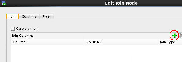
B. In the Edit Join Column window:
The Edit Join Column window should now look like this:
C. Click OK in the Edit Join Column window to save the join definition.
Then, using the Columns tab of the Edit Join Node window, remove the USERNAME column from the CUSTOMER_TARGET source.
A. First, perform the following:
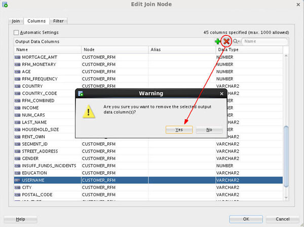
Result: Now, the total number of specified columns should be 44.
B .Finally, click OK in the Edit Join Node window.
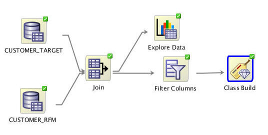
The workflow should now look like something like this. Notice that the warning indicator is no longer displayed on the Join node.

Explore the Source Data
You can use an Explore Data node to further examine the source data. You can also use a Graph node to visualize data. Although these are optional steps, Oracle Data Miner provides these tools to enable you to verify if the selected data meets the criteria to solve the stated business problem.
Follow these steps:
Open the Data category once again, and drop an Explore Data node on the workflow, like this:
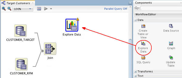
Result: A new Explore Data node appears in the workflow pane, as shown.
Notes:
To connect the joined data sources and explore the data nodes, use the following instructions:
A. Right-click the Join node, select Connect from the pop-up menu, drag the pointer to the Explore Data node, and click.
The result should look something like this:
Next, select a "Group By" attribute for the Explore Data node.
A. Double-click the Explore Data node to display the Edit Explore Data Node window.
B. In the Group By list, select the IS_TARGET attribute, as shown here:
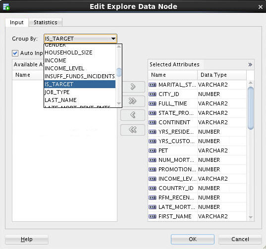
C. Then, click OK.
Note: The Selected Attributes window also allows you to remove (or re-add) any attributes from the source data.
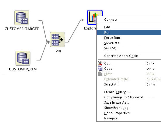
Next, right-click the Explore Data node and select Run.
Result:
Note: When you run any process from the workflow canvas, the steps that you have specified are executed by the Oracle Data Miner Server.
To see results from the Explore Data node, perform the following:
A. Right-click the Explore Data node and select View Data from the menu.
Result: A new tab opens for the Explore Data node, as shown below.
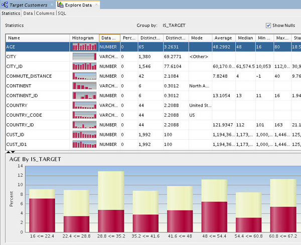
Notes:
B. Select any of the attributes in the Name list to display the associated histogram in the bottom window.
C. When you are done examining the source data, dismiss the Expore Data tab by clicking the Close icon (X).
Save the workflow by clicking the Save All icon in main toolbar.
Create Classification Models
As stated in the Overview section of this tutorial, classification models are used to predict individual behavior. In this scenario, you want to predict which customers are most likely to be the best customers in terms of sales. Therefore, you will specify a classification model.
When using Oracle Data Miner, a classification model node creates four models using different algorithms, and all of the models in the classification node have the same target and Case ID. This default behavior makes it easier to figure out which algorithm gives the best predictions. Here, you define a Classification node that uses all algorithms for the model.
Notes:
Therefore, before adding the Classification model node, add a Filter Columns node.
A. Collapse the Data category, and expand the Transforms category in the Components tab:
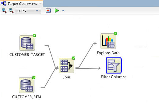
B. Drag and drop a Filter Columns node from the Components tab to the Workflow pane, like this
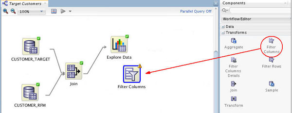
C. Connect the Join node to the Filter node like this:
Next, edit the node to specify Attribute Importance for the Target field.
A. Double-click the Filter Columns node, and then click the Settings button in the top-right corner of the Edit Filter Columns Node window.
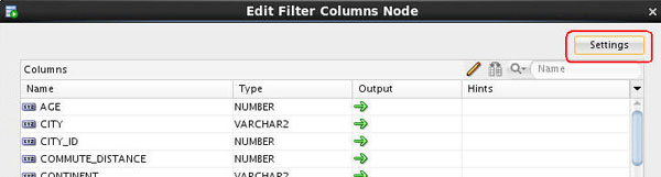
B. In the Define Filter Column Settings window, enable the Attribute Importance option, and then select IS_TARGET from the Target drop-down list, as shown here:
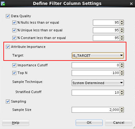
Note: Accept all of the other derfault settings.
C. Click OK.
D. Finally, click OK in the Edit Filter Columns Node window to save the Attribute Importance specification.
Now, run the Filter Columns node to see the results of the Attribute Importance specification.
A. Right-click the Filter Columns node and select Run from the menu.
B. When the Run process is complete (green check mark in node border), double-click the Filter Columns node to view the Attribute Importance recommendations.
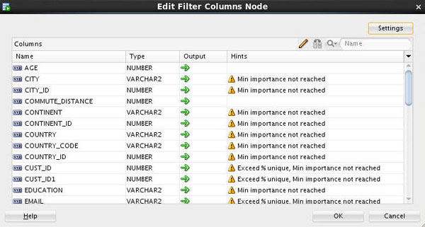
Notes:
C. Select all of the rows in the list. Then, click the Apply Recommended Ouput Settings tool, as shown here:
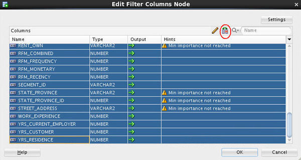
Result: All of the recommended columns are filtered out (a red "x" is added to the Output designation for each column).
E. Now, click the Output designation for the CUST_ID column, so that it will be passed forward as a column in the modeling process (the red "x" dissapears). The Filter Columns list should now look like this:
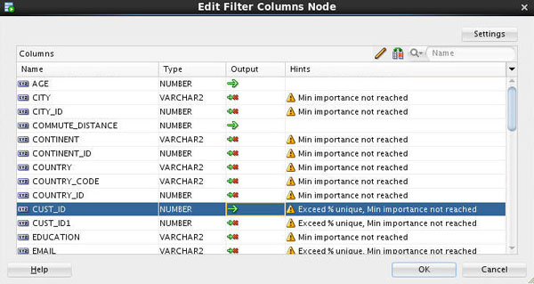
F. Click OK to close the Edit Filter Columns Node window.
Next, add the Classification node.
A. First, collapse the Transforms category, and expand the Models category in the Components tab:
B. Then, drag and drop the Classification node from the Components tab to the Workflow pane:
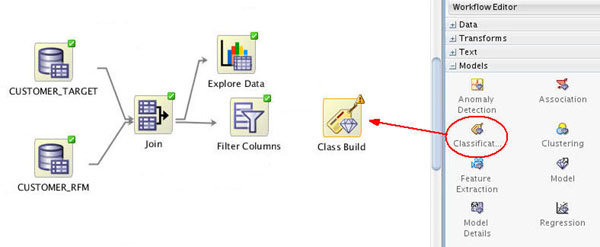
Result: A node with the name "Class Build" appears in the workflow:
Notes:
First, connect the Filter Columns node to the Class Build node using the same technique described previously.
Result: the Edit Classification Build Node window appears.
Next, select the Build tab in the Edit Classification Build Node window.
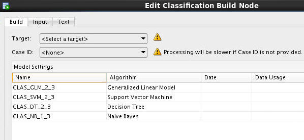
Notes:
In the Build tab, perform the following:
A. Select IS_TARGET as the Target attribute.
B. Select CUST_ID as the Case ID attribute.
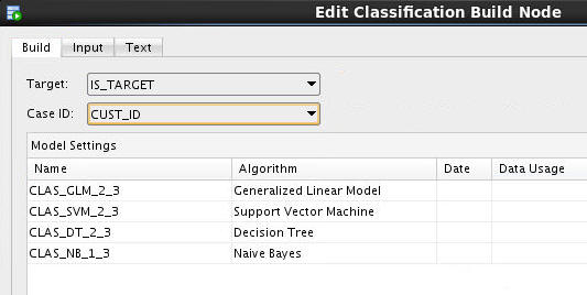
Notes:
C. Click OK in the Edit Classification Build Node window to save your changes.
Result: The classification build node is ready to run.
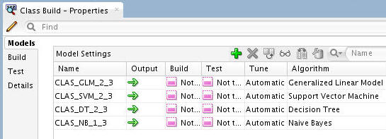
Note: In the Models section of the Properties tab, you can see the current status for each of the selected algorithms, as shown below:
Save the workflow by clicking the Save All icon.
Build the Models
In this topic, you build the selected models against the source data. This operation is also called “training”, and the model is said to “learn” from the training data.
A common data mining practice is to build (or train) your model against part of the source data, and then to test the model against the remaining portion of your data. By default, Oracle Data Miner uses this approach, at a 40/60 split.
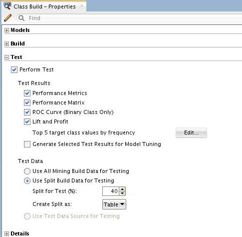
Before building the models, select Class Build node and expand the Test section of the Properties tab. In the Test section, you can specify:
Here, the default settings for the test phase are shown.
Next, you build the models.
Right-click the Class Build node and select Run from the pop-up menu.
Notes:
When the build is complete, all nodes contain a green check mark in the node border.
In addition, you can view several pieces of information about the build using the property inspectory.
Select the classification build node in the workflow, and then select the Models section in the Properties tab.
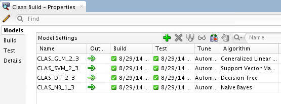
Notes:
Compare the Models
After you build/train the selected models, you can view and evaluate the results for all of the models in a comparative format. Here, you compare the relative results of all four classification models.
Follow these steps:
Right-click the classification build node and select Compare Test Results from the menu.
Results: A Class Build display tab opens, showing a graphical comparison of the four models in the Performance tab, as shown here:
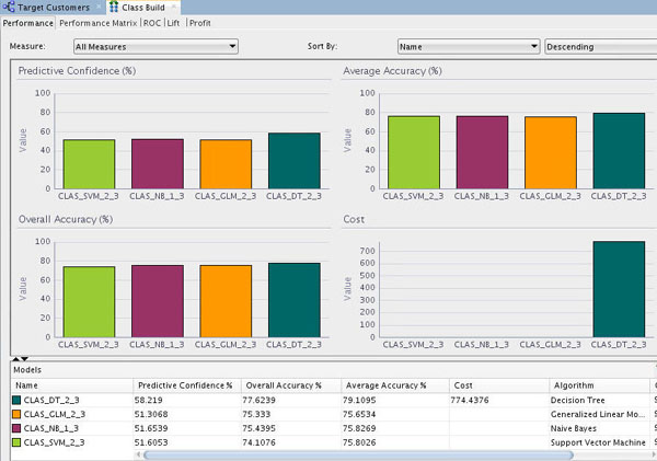
Notes:
Since the sample data set is very small, the numbers you get may differ slightly from those shown in the tutorial example. In addition, the histogram colors that you see may be different then those shown in this example.
Select the Lift tab. Then, select a Target Value of 1 (yes), in the upper-right side of the graph.
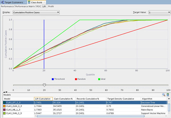
Notes:
Using the example shown above at the 20th quantile, the Decision Tree model has the highest Lift Cumulative and Gain Cumulative %, although all of the models are very close in terms of these measurements.
In the Lift tab, you can move the Quanitile measure point line along the X axis of the graph by using the slider tool, as shown below. The data in the Models pane at the bottom updates automatically as you move the slider left or right.
Note the following, as shown in the image below:
Next, select the Performance Matrix tab.
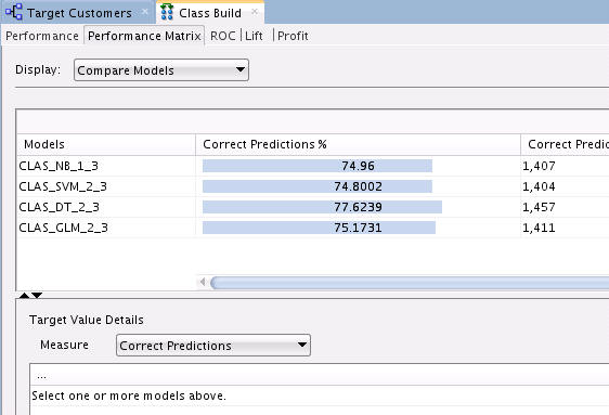
Notes:
Compare the details for the three top models.
First, select the GLM model to view the Target Value Details for this model. Recall that the "Target Value" for each of the models is the IS_TARGET attribute.
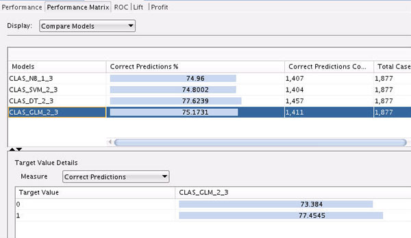
Notes: The GLM model indicates a 73.38% correct prediction outcome for customers that aren't considered targets and a 77.45% correct prediction outcome for customers that are considered targets.
Next, select the NB model to view the Target Value Details for this model. Recall that the "Target Value" for each of the models is the IS_TARGET attribute.
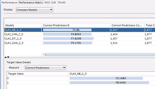
Notes: The NB model indicates a 72.15% correct prediction outcome for customers that aren't considered targets and a 78.55% correct prediction outcome for customers that are considered targets.
Finally, select the DT model.
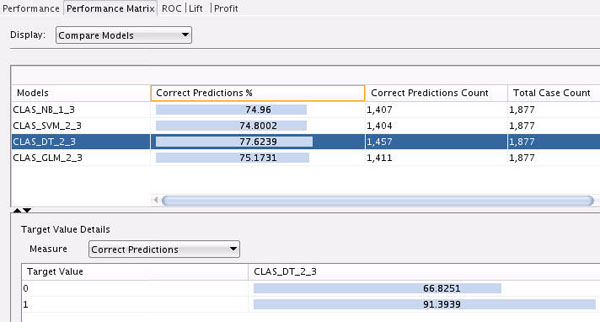
Notes: The DT model indicates a 66.8% correct prediction outcome for customers that aren't considered targets, and a 91.4% correct prediction outcome for customers that are considered targets.
After considering the initial analysis, you decide to investigate the Decision Tree model more closely. Dismiss the Class Build tabbed window.
Select and Examine a Specific Model
Using the analysis performed in the previous topic, the Decision Tree model is selected for further analysis.
Follow these steps to examine the Decision Tree model
Back in the workflow pane, right-click the Class Build node again, and select View Models > CLAS_DT_2_3 (Note: The exact name of your Decision Tree model may be different).
Result: A window opens that displays a graphical presentation of the Decision Tree.
The interface provides several methods of viewing navigation:
For example, set the the primary viewer window for the decision tree to 75% zoom.
First, navigate to and select Node 5.
Notes:
Notes:
Next, scroll down to the bottom of the tree. There are two leaf nodes that indicate a prediction of 1 (part of the target group) - nodes 17 and 15.
A. Select Node 17, as shown here:
Notes:
Now, select Node 15, as shown here:
Notes:
Dismiss the Decision Tree display tab (CLAS_DT_2_3).
Apply the Model
In this topic, you apply the Decision Tree model and then create a table to display the results. You "apply" a model in order to make predictions - in this case to predict which customers are likely to buy insurance.
To apply a model, you perform the following steps:
Follow these steps to apply the model and display the results:
In the workflow, select the Class Build node. Then, using the Models section of the Properties tab, deselect all of the models except for the DT model.
To deselect a model, click the large green arrow in the model's Output column. This action adds a small red "x" to the column, indicating that the model will not be used in the next build.
When you finish, the Models tab of the Property Inspector should look like this:
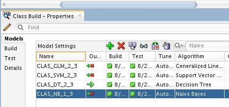
Note: Now, only the DT model will be passed to subsequent nodes.
Next, add a new Data Source node in the workflow. Note: Even though we are using the same table as the "Apply" data source, you must still add a second data source node to the workflow.
A. From the Data category in the Components tab, drag and drop a Data Source node to the workflow canvas, as shown below. The Define Data Source wizard opens automatically.
B. In Step 1 of the wizard, select ODMUSER.CUSTOMER_PROSPECTS from the list and click Finish.
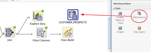
Result: A new data souce node appears on the workflow canvas, with the name CUSTOMER_PROSPECTS.
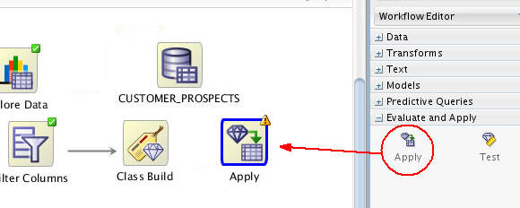
Next, expand the Evaluate and Apply category in the Components tab.
Drag and drop the Apply node to the workflow canvas, like this:
Using the Details tab of the Property Inspectory, rename the Apply node to Apply Model.
Using the techniques described previously, connect the Class Build node to the Apply Model node, like this
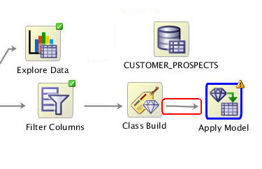
Then, connect theCUSTOMER_PROSPECTS node to the Apply Model node:
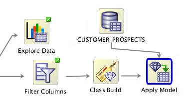
Notes:
Before you run the apply model node, consider the resulting output. By default, an apply node creates two columns of information for each customer:
However, you really want to know this information for each customer, so that you can readily associate the predictive information with a given customer.
To get this information, you need to add a third column to the apply output: CUST_ID. Follow these instructions to add the customer identifier to the output:
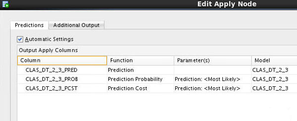
A. Right-click the Apply Model node and select Edit.
Result: The Edit Apply Node window appears. Notice that the Prediction, Prediction Probability, and Prediction Cost columns are defined automatically in the Predictions tab.
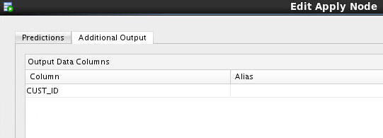
B. Select the Additional Output tab, and then click the green "+" sign, like this:
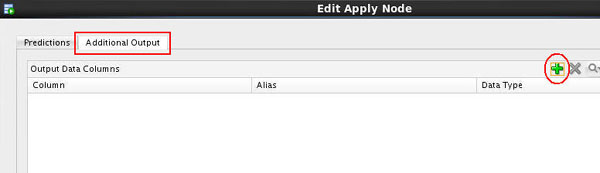
C. In the Edit Output Data Column Dialog:
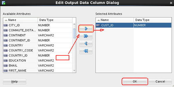
Result: the CUST_ID column is added to the Additional Output tab, as shown here:
Also, notice that the default column order for output is to place the data columns first, and the prediction columns after. You can switch this order if desired.
D. Finally, click OK in the Edit Apply Node window to save your changes.
Now, you are ready to apply the model. Right-click the Apply Model node and select Run from the menu.
Result: As before, the workflow document is automatically saved, and small green gear icons appear in each of the nodes that are being processed. In addition, the execution status is shown at the top of the workflow pane.
When the process is complete, green check mark icons are displayed in the border of all workflow nodes to indicate that the server process completed successfully.
Optionally, you can create a database table to store the model prediction results (defined in the "Apply Model" node).
The table may be used for any number of reasons. For example, an application could read the predictions from that table, and suggest an appropriate response, like sending the customer a letter, offering the customer a discount, or some other appropriate action.
To create a table of model prediction results, perform the following:
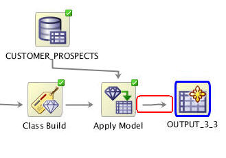
A. Using the Data category in the Components pane, drag the Create Table or View node to the workflow window, like this:
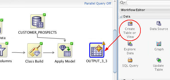
Result: An OUTPUT node is created (the name of your OUTPUT node may be different than shown in the example)..
B. Connect the Apply Model node to the OUTPUT node.
C. To specify a name for the table that will be created (otherwise, Data Miner will create a default name), do the following:
1. Right-click the OUTPUT node and select Edit from the menu.
2. In the Edit Create Table or View Node window, change the default table name to DT_PREDICTIONS, as shown here:
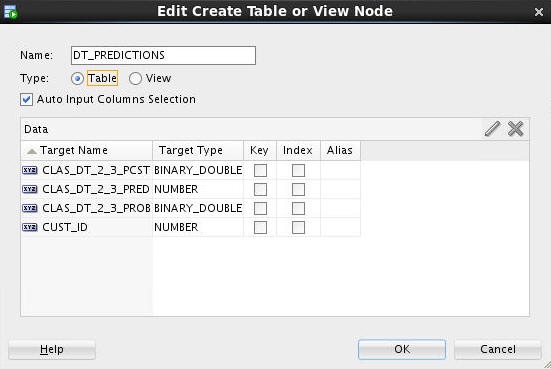
3. Then, click OK.
D. Lastly, right-click the DT_PREDICTIONS node and select Run from the menu.
Result: The workflow document is automatically saved when the process is executed. When complete, all nodes contain a green check mark in the border, like this:
Note: After you run the OUTPUT node (DT_PREDICTIONS), the table is created in your schema.
To view the results:
A. Right-click the DT_PREDICTIONS Table node and select View Data from the Menu.
Result: A new tab opens with the contents of the table:
B. Click Apply Sort to view the results:
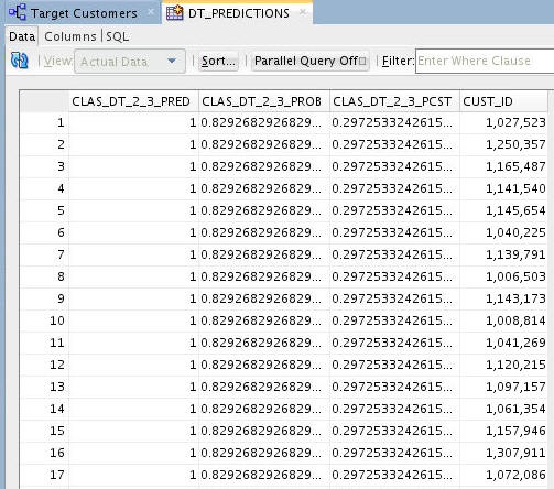
Notes:
C. When you are done viewing the results, dismiss the tab for the DT_PREDICTIONS table, and click Save All.
Summary
- Identify Data Miner interface components
- Create a Data Miner project
- Build a Workflow document that uses Classification models to predict customer behavior
- See the Oracle Data Mining and Oracle Advanced Analytics pages on OTN.
- Refer to additional OBEs in the Oracle Learning Library
- See the Data Mining Concepts manuals: Oracle Database 12c Release 1 (12.1)
In this lesson, you examined and solved a "Classification" prediction data mining business problem by using the Oracle Data Miner graphical user interface, which is included as an extension to SQL Developer, version 4.0.
In this tutorial, you have learned how to:
Resources
To learn more about Oracle Data Mining:
Credits
Lead Curriculum Developer: Brian Pottle
Other Contributors: Charlie Berger, Mark Kelly, Margaret Taft, Kathy Talyor
To help navigate this Oracle by Example, note the following:
- Hiding Header Buttons:
- Click the Title to hide the buttons in the header. To show the buttons again, simply click the Title again.
- Topic List Button:
- A list of all the topics. Click one of the topics to navigate to that section.
- Expand/Collapse All Topics:
- To show/hide all the detail for all the sections. By default, all topics are collapsed
- Show/Hide All Images:
- To show/hide all the screenshots. By default, all images are displayed.
- Print:
- To print the content. The content currently displayed or hidden will be printed.
To navigate to a particular section in this tutorial, select the topic from the list.