This tutorial illustrates how you can securely analyze data
across the big data platform - whether that data resides in
Oracle Database 12c, Hadoop, Oracle NoSQL Database or a
combination of these sources. Importantly, you will be able to
leverage your existing Oracle skill sets and applications to
gain these insights. Oracle Big Data SQL allows you to apply
Oracle's rich SQL dialect and security policies across the data
platform - greatly simplifying the ability to gain insights from
all your data.
Note, there are two parts to Big Data SQL: 1) enhanced Oracle
Database 12c external tables and 2) Oracle Big Data SQL Servers
on the Oracle Big Data Appliance or DIY Hadoop Clusters (see Big
Data SQL Datasheet for supported deployments). On the
Hadoop cluster, Big Data SQL Cell Servers apply SmartScan over
data stored in HDFS in order to achieve fast performance (see
this blog
post for details). The Oracle Big Data Lite Virtual
Machine used for this lab does not have Big Data SQL Cell Server
installed.
Time to Complete
Approximately 90 mins
Prerequisites
This tutorial requires Oracle BIg Data Lite Virtual Machine
(VM). You can download the VM from the Big
Data Lite page on OTN.
Before starting this lesson, perform the following:
After starting Big Data Lite, ensure the following services
are started by using the Start/Stop Services application found
on the Linux desktop:
ORCL
Zookeeper
HDFS
Hive
NoSQL
YARN
Note the started services have an * next to their name:
Using the right-mouse menu, save the following two files to
a directory on the machine where SQL Developer is installed: bigdatasql_hol_otn_setup.sql
and bigdatasql_hol.sql.
Remember this location - you will open these files in SQL
Developer in just a minute! NOTE: Use the 'Save Link As'
option in the menu.
Launch SQL Developer from the Desktop Toolbar menu, as shown
here:
In SQL Developer, open both files.
Select the bigdatasql_hol_otn_setup.sql
script, and then click the Run Script tool
in the SQL Developer, as shown below. When prompted for a
connection, select the moviedemo connection
and click OK. This will complete the setup
for this tutorial.
Close the bigdatasql_hol_otn_setup.sql script.
Next, in the bigdatasql_hol.sql script,
multi-select the drop statements
at the top of the script and click the Run Statement
tool, as shown here:
Note: Ignore any errors generated by these statements.
Leave the bigdatasql_hol.sql script open in SQL Developer,
as it contains all of code examples that are referenced in
this tutorial.
Introduction
This tutorial is divided into the following sections:
Review the Scenario
Configuring Oracle Big Data SQL
Create Oracle Tables Over an HDFS Sourced Application Log
Leverage the Hive Metastore to Access Data in Hadoop and
Oracle NoSQL Database
Applying Oracle Database Security Policies Across the Big
Data Platform
Using Oracle Analytic SQL Across All Your Data
Using SQL Pattern Matching on your web log data
Scenario
Oracle MoviePlex is an online movie streaming company.
Every user that accesses the site is presented with his/her own
movie recommendations based on past viewing activity. This
list of recommended movies is updated frequently and is part of
the user's profile. Oracle NoSQL Database stores these
profiles - delivering application query requests with very low
latency for large user communities. Additionally, the web
site collects every customer interaction in massive JSON
formatted log files. By unlocking the information
contained in that activity data and combining it with
recommendation data and enterprise data in its data warehouse,
the company will be able to enrich its understanding of customer
behavior, the effectiveness of product offers, the organization
of web site content, and more.
The company is using Oracle's Big Data Management System to
unify their data platform and facilitate these analyses.
Oracle Big Data Management System unifies the data platform by
providing a common query language, management platform and
security framework across Hadoop, NoSQL and Oracle
Database. Oracle Big Data SQL is a key component of the
platform. It enables Oracle Database 12c to seamlessly
query data in Hadoop and NoSQL using Oracle's rich SQL
dialect. Data stored in Hadoop or Oracle NoSQL Database is
queried in exactly the same way as all other data in Oracle
Database. This means that users can begin to gain insights
from these new sources using their existing skill sets and
applications.
For Oracle MoviePlex, every click on its web site is streamed
into HDFS. After the data lands in HDFS, it is immediately
accessible to Oracle Database users through Oracle Big Data SQL.
In addition, the recommendation data in Oracle NoSQL Database is
also accessible thru Oracle Big Data SQL. In this
hands-on, you will learn how to combine the "click data" stored
in HDFS with recommendation data in NoSQL Database and revenue
data in Oracle Database to better understand the shopping and
purchasing patterns of customers visiting the site.
Let's begin the tutorial by reviewing how access to the BDA is
configured in Oracle Database.
Part 1 - Configuring Oracle Big Data SQL
In this section, you learn how to configure Oracle Big Data
SQL. This configuration process enables Oracle Database
12c to query data in Hadoop or Oracle NoSQL Database.
Configuration Tasks
As mentioned in the overview, this VM uses enhanced
external tables in Oracle Database 12c to access data in
HDFS and Oracle NoSQL Database. It does not have the
Big Data SQL Server Cells installed. In a true
Oracle Big Data environment, there are two installation
tasks:
Install Oracle Big Data SQL on the Hadoop
cluster. This step sets up a Big Data SQL Server
Cells on each node A - enabling SmartScan on local data.
For Oracle Database 12c, run the Big Data SQL
installation script on each Oracle database node.
This step sets up connectivity from Oracle Database to
the Big Data SQL Server Cells on the Hadoop
Cluster. It also includes installing a Hadoop
client, configuration directories and files, Big Data
SQL Agent, Oracle directory objects and more.
Let's review some of the important elements that are
produced in the second configuration task.
Review the Common and Cluster Directories
Two file system directories -- the Common and Cluster
directories -- are set up in the Oracle Database home.
These directories store configuration files that enable
the Exadata Server to connect to the BDA. A short
description of each follows.
Common Directory
The Common directory contains a few subdirectories and
an important file, named bigdata.properties.
This file stores configuration information that is
common to all BDA clusters. Specifically, it
contains property-value pairs used to configure the JVM
and identify a default cluster.
The bigdata.properties file must be
accessible to the operating system user under which the
Oracle Database runs.
Cluster Directory
The Cluster directory contains configuration files
required to connect to a specific BDA cluster.
In addition, the Cluster directory must be a
subdirectory of the Common directory - and the name of
the directory is important: It is the name that you will
use to identify the cluster. This will be described in
more detail later.
First, let's review the Common Directory's bigdata.properties
file:
Launch a Terminal window using the Desktop toolbar.
(SQL Developer should also be open.)
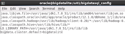
In the Terminal window, change to the Common
directory location, and then view the contents of
the bigdata.properties file.
Enter the following commands at the prompt:
cd
/u01/bigdatasql_config/
cat bigdata.properties
Result: The output of the commands will look
similar to the following:
Notes:
The properties, which are not specific to a
hadoop cluster, include items such as the location
of the Java VM, classpaths and the
LD_LIBRARY_PATH.
In addition, the last line of the file specifies
the default cluster property - in this case bigdatalite.
As you will see later, the default cluster
simplifies the definition of Oracle tables that
are accessing data in Hadoop.
In our hands-on lab, there is a single
cluster: bigdatalite.
The bigdatalite subdirectory
contains the configuration files for the bigdatalite
cluster.
The name of the cluster must match the name of
the subdirectory (and it is case sensitive!).
Next, let's review the contents of the Cluster
Directory.
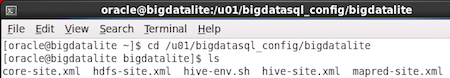
Using the Terminal window, change to the Cluster
directory and view it's contents by executing the
following commands at the prompt:
cd
/u01/bigdatasql_config/bigdatalite
ls
Result: The output of the commands above will look
similar to the following:
Notes:
These are the files required to connect Oracle
Database to HDFS and to Hive.
Each cluster will have its own directory - with
configuration files specific to that cluster.
Oracle directory objects that correspond to these
file system directories are
created by the install process.
Review Oracle Directory Objects
As previously shown, the configuration files have been
saved to the file system. The installation process
creates corresponding Oracle directory objects that
point to these folders.
The Oracle directory objects have a specific naming
convention:
ORACLE_BIGDATA_CONFIG : the Oracle directory object
that references the Common Directory
ORACLE_BIGDATA_CL_bigdatalite : the Oracle directory
object that references the Cluster Directory. The
naming convention for this directory is as follows:
Cluster Directory name begins with
ORACLE_BIGDATA_CL_
Followed by the cluster name (i.e.
"bigdatalite"). This name is case sensitive
(so don't forget quotes for lowercase names!) and is
limited to 15 characters.
Must match the physical directory name in the file
system (repeat: it's case sensitive!).
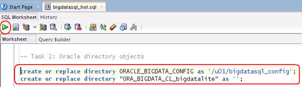
Review these Oracle directory objects:
In SQL Developer, using the bigdatasql_hol script
file, execute the following statement:
Notes:
In SQL Developer, use the Run
Statement tool (shown above) to run
one or more selected statements.
The directory object is case sensitive.
In our example, the bigdatalite cluster is lower
case and was created by the install script using
the following command:
create or
replace directory "ORA_BIGDATA_CL_bigdatalite"
as '';
Notice that there is no location specified for
the Cluster Directory. It is expected that
the directory will:
Be a subdirectory of ORACLE_BIGDATA_CONFIG
Use the cluster name as identified by the
Oracle directory object.
Review Oracle Big Data SQL Agent
In addition to creating the Oracle directory
objects, Big Data SQL Agents are also created by
the install script:
This multi-threaded agent bridges the metadata
between Oracle Database and Hadoop. It
launches a single JVM - instead of one for every
process (which can be quite slow).
If the MTA were not already set up, you would
use the following commands to create it:
create public
database link BDSQL$_bigdatalite using
'extproc_connection_data';
create public database link
BDSQL$_DEFAULT_CLUSTER using
'extproc_connection_data';
Now that we have reviewed the configuration, lets
create Oracle tables that access data in HDFS and Oracle
NoSQL Database!
Part 2 - Create Oracle Table Over Application Log
In this section, you will create an Oracle table over data
stored in HDFS and then query that data. This example
will use the ORACLE_HDFS driver; it will not
leverage metadata stored in the Hive Catalog.
Review Application Log Stored in
HDFS
The movie application streamed data into HDFS - specifically
into the following directory: /user/oracle/moviework/applog_json.
Let's review that log data:
Open a terminal window.
Execute the following command to
review the log file stored in HDFS:
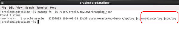
hadoop fs -ls
/user/oracle/moviework/applog_json
Result: You should see the following output:
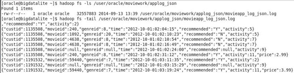
Now, view the contents of the file, execute the
following command:
Notice the file contains every click that has taken
place on the web site. The JSON log captures the
following information about each interaction:
custid:
the customer accessing the site
movieid:
the movie that the user clicked on
genreid:
the genre that the movie belongs to
time:
when the activity occurred
recommended:
did the customer click on a recommended movie?
activity:
a code for the various activities that can take
place, including log in/out, view a movie, purchase
a movie, show movie listings, etc.
price:
the price of a purchased movie
Create Oracle Table Over
Application Log
Now that you have reviewed the source data, create an
Oracle table over the file. This table will be very
simple: a single column where each record contains a
JSON document. You will then user Oracle SQL to
easily parse the JSON fields found in each document:
Go to the SQL Worksheet in SQL Developer and execute
the following SQL statement (Note: These statements
are all in the bigdatasql_hol.sql
script):
Notice in the code above that Oracle external tables
have been enhanced to natively understand data stored
on the BDA. Specifically, the following attributes are
leveraged:
Access
driver ORACLE_HDFS indicates that
the data is stored in HDFS.
LOCATION
identifies the HDFS directory (or file or
directories) that contains the source data for the
table
The DEFAULT
DIRECTORY contains log files that are
generated by the external table (if logging is
enabled)
The REJECT
LIMIT applies to each parallel query
slave that is executing the query.
Execute the following command to
review the data in the table
movielog
SELECT * FROM movielog
WHERE rownum < 20;
Result: The output will look similar to our previous
tail statement. A record is returned each JSON
document.
There are numerous options that can be applied to the
external table that impact how the data is queried and
processed. Let's take a look at a couple of
these options. Create the table movielog_plus
by using the following DDL command:
First, the click column has been
changed to a VARCHAR2(40).
Clearly, this is going to be a problem; the length
of a JSON document exceeds that size. There
are numerous ways to handle this situation,
including:
Generate an error and then either reject the
record, set its value to null or replace it with
an alternate value.
Simply truncate the data. Here, we are
truncating the data. And, we have applied
this truncate action to all columns in the
table; you can also specify the individual
column(s) to truncate.
Second, a cluster bigdatalite has
been specified. This cluster will be used
instead of the default (which in this case happens
to be the same). Currently a given session may
only connect to a single cluster.
Execute the following command to review the data in
the table movielog_plus:
SELECT * FROM
movielog_plus WHERE rownum < 20;
Note: Each JSON document is truncated based on the
size of the Oracle table column (40
characters). In practice, truncating a JSON
document is not very useful, but this example
illustrates the point.
Oracle Database 12c (12.1.0.2)
includes native JSON support. This allows queries
to easily extract attribute data from JSON
documents. Run the following query in SQL
Developer:
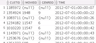
SELECT m.click.custid,
m.click.movieid, m.click.genreid, m.click.time
FROM movielog m
WHERE rownum < 20;
Result: The query output looks like this:
Notes:
The column specification in the select list is a
full path to the JSON attribute.
The specification starts with the table alias
("m" - note: this is required!), followed by the
column name ("click"), and then a case sensitive
JSON path (e.g. "genreId").
One of the key strengths of Oracle Big Data SQL is
the ability to answer questions that combine data from
Oracle Database and Hadoop. Combine the "click"
data with data sourced from the movie
dimension table, by executing the following command:
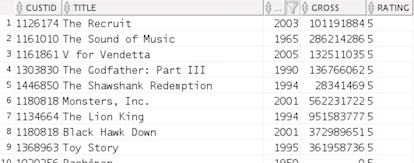
SELECT f.click.custid,
m.title, m.year, m.gross, f.click.rating
FROM movielog f, movie m
WHERE f.click.movieid = m.movie_id
AND f.click.rating > 4;
Result: The query results will look similar in
structure to the following (your record output may be
in a different order):
Note: The output above enables us to see how a given
customer's ratings on the web site compared to the
movies' gross revenues.
Execute the following command to
create a view to simplify queries against the JSON data.
This view will also be useful in subsequent exercises
when security policies are applied to the table:
CREATE OR REPLACE VIEW
movielog_v AS
SELECT
CAST(m.click.custid AS NUMBER)
custid,
CAST(m.click.movieid AS NUMBER) movieid,
CAST(m.click.activity AS NUMBER) activity,
CAST(m.click.genreid AS NUMBER) genreid,
CAST(m.click.recommended AS VARCHAR2(1))
recommended,
CAST(m.click.time AS VARCHAR2(20)) time,
CAST(m.click.rating AS NUMBER) rating,
CAST(m.click.price AS NUMBER) price
FROM movielog m;
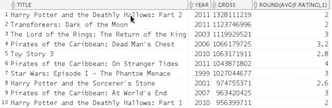
Now, execute the following command to
find how Oracle MoviePlex average ratings compare to top
10 grossing movies:
SELECT m.title, m.year,
m.gross, round(avg(f.rating), 1)
FROM movielog_v f, movie m
WHERE f.movieid = m.movie_id
GROUP BY m.title, m.year, m.gross
ORDER BY m.gross desc
FETCH FIRST 10 ROWS ONLY;
Result: The output looks like this:
Note: The data indicates that MoviePlex users aren't
necessarily enjoying blockbuster movies.
Summary:
In a matter of minutes, you were able to create and query
Oracle Database tables over data sourced in HDFS - and
then join that data with other Oracle Database
tables.
Next, we will leverage metadata already available in the
Hive Metastore to make it even easier to query complex
data in Hadoop.
Part 3 - Leverage the Hive Metastore to Access Data in
Hadoop & Oracle NoSQL Database
Hive enables SQL access to data stored in Hadoop and NoSQL
stores. There are two parts to Hive: the Hive execution
engine and the Hive Metastore.
The Hive execution engine launches MapReduce job(s) based on
the SQL that has been issued. MapReduce is a batch
processing framework and is not intended for interactive query
and analysis - but it is extremely useful for querying massive
data sets using the well understood SQL language.
Importantly, no coding is required (Java, Pig, etc.). The
SQL
supported by Hive is still limited (SQL92), but
improvements are being made over time.
The Hive Metastore has become the standard metadata repository
for data stored in Hadoop. It contains the definitions of tables
(table name, columns and data types), the location of data files
(e.g. directory in HDFS), and the routines required parse that
data (e.g. StorageHandlers, InputFormats and SerDes). The
data accessed thru Hive does not have to be stored in
Hadoop. For example, Oracle NoSQL Database offers a
StorageHandler that makes its data accessible thru Hive.
This capability will be leveraged by Oracle Big Data SQL.
There are many query execution engines that use the Hive
Metastore while bypassing the Hive execution engine.
Oracle Big Data SQL is an example of such an engine. This means
that the same metadata can be shared across multiple products
(e.g. Hive, Oracle Big Data SQL, Impala, Pig, Spark SQL,
etc.); you will see an example of this in action in the
following exercises.
Let's begin by reviewing the tables that have been defined in
Hive. After reviewing these hive definitions, we'll create
tables in the Oracle Database that will query the underlying
Hive data stored in HDFS and Oracle NoSQL Database:
Review Tables Stored in Hive
Tables in Hive are organized into databases. In
our example, several tables have been created in the
default database. Connect to Hive and investigate these
tables.
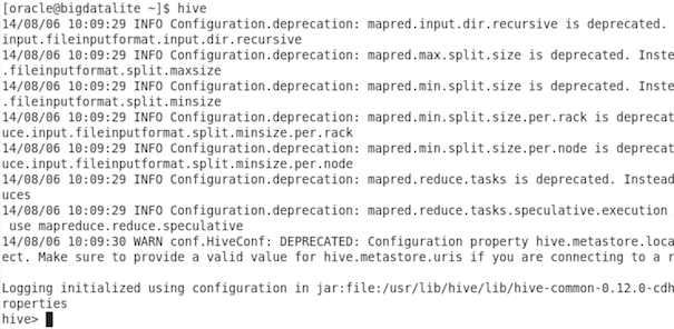
Open a terminal window and execute the following
command at the command prompt:
bee
Result: This command is a shortcut for running
beeline - a Hive JDBC client (see /opt/bin/bee).
Beeline is a very basic Hive command line interface
(CLI).
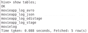
At the prompt, enter the following
command to display the list of tables in the default
database:
show tables;
Result: As shown in the output, several tables have
been defined in the database. There are tables defined
over Avro data, JSON data and tab delimited text
files.
Let's review two tables that have been defined over JSON
data.
The first table is very simple and is equivalent to
the external table that was defined in Oracle Database
in the previous exercise. Review the definition
of the table by executing the following command at the
prompt:
show create table
movielog;
Result: The DDL for the table is displayed.
Notes:
There is a single string column called click
- and the table is referring to data stored in the /user/oracle/moviework/applog_json
folder.
There is no special processing of the JSON data;
i.e. no routine is transforming the attributes into
columns. The table is simply displaying the JSON as
a line of text.
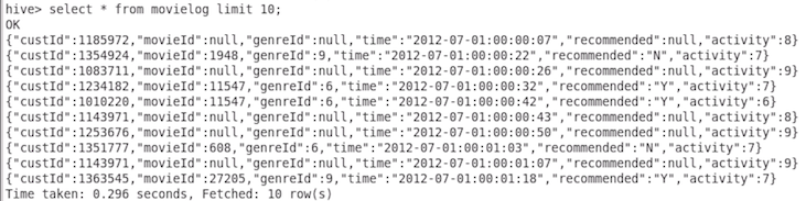
Next, query the data in the movielog
table by executing the following command:
select * from movielog
limit 10;
Result: The follow output is produced:
Notes:
Because there are no columns in the select list
and no filters applied, the query simply scans the
file and returning the results.
No MapReduce job is executed.
There are more useful ways to query the JSON
data. The next steps will show how Hive can
parse the JSON data using a serializer/deserializer -
or SerDe.
The second table queries that same file - however
this time it is using a SerDe that will translate the
attributes into columns. Review the definition of the
table by executing the following command:
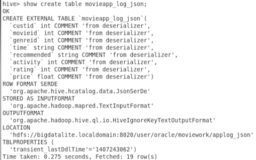
show create table
movieapp_log_json;
Result: The DDL for the second table is shown.
Notes:
There are columns defined for each field in the
JSON document - making it much easier to understand
and query the data.
A java class org.apache.hive.hcatalog.data.JsonSerDe
is used to deserialize the JSON file.
This is also an illustration of Hadoop's schema on
read paradigm; a file is stored in HDFS, but there is
no schema associated with it until that file is
read. Our examples are using two different
schemas to read that same data; these schemas are
encapsulated by the Hive tables movielog
and movieapp_log_json.
Execute the following query against the
movieapp_log_json table to find movies that were
highly rated:
SELECT movieid,
AVG(rating) AS avg_rating
FROM movieapp_log_json
WHERE rating IS NOT NULL
GROUP BY movieid
ORDER BY avg_rating DESC, movieid ASC
LIMIT 25;
Result: The following output is generated (the query
may take a moment to return these results).
Note: This is a much better way to query and view
the data than in our previous table.
The Hive query execution engine converted this
query into MapReduce jobs.
The author of the query does not need to worry
about the underlying implementation - Hive handles
this automatically.
Review a third table called recommendation.
This table is in the moviework database and is
defined over an Oracle NoSQL Database table that
contains movie recommendations for each user:
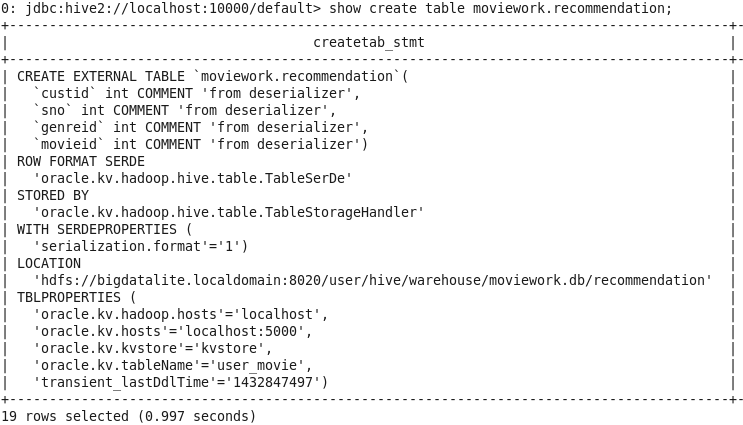
show create table
moviework.recommendation;
Result: The DDL for the third table is shown.
Notes:
The TBLPROPERTIES describe the connection
details for the Oracle NoSQL Database instance
An Oracle NoSQL DB storage handler oracle.kv.hadoop.hive.table.TableStorageHandler
provides access to the underlying data store
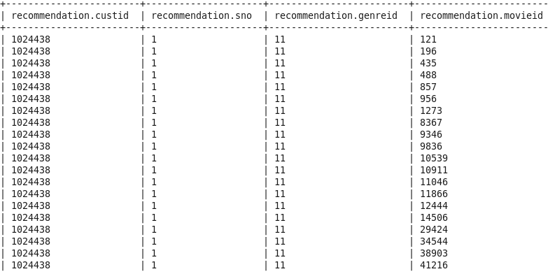
Execute the
following query against the recommendation table to
view genres and movies recommended for users:
SELECT * FROM
moviework.recommendation LIMIT 20;
At the prompt, execute the !exit;
command to close beeline
Leverage Hive Metadata When
Creating Oracle Tables
Oracle Big Data SQL is able to leverage the Hive
metadata when creating and querying tables.
In this section, you will create Oracle tables over
three Hive tables: movieapp_log_json,
movieapp_log_avro and recommendation.
Oracle Big Data SQL will utilize the existing
StorageHandlers and SerDes required to process this data.
Go to Oracle SQL Developer. Create a table over
the Hive movieapp_log_json table using the following
DDL:
Notice the new ORACLE_HIVE access
driver type. This access driver invokes Oracle
Big Data SQL at query compilation time to retrieve the
metadata details from the Hive Metastore. By
default, it will query the metastore for a table name
that matches the name of the external table: movieapp_log_json.
As you will see later, this default can be overridden
using ACCESS PARAMETERS.
Query the table using the following select statement:
SELECT * FROM
movieapp_log_json WHERE rating > 4
Result: The query output is shown here:
Notes:
As mentioned earlier, at query compilation time,
Oracle Big Data SQL queries the Hive Metastore for
all the information required to select data.
This metadata includes the location of the data and
the classes required to process the data (e.g.
StorageHandlers, InputFormats and SerDes).
In this example, Oracle Big Data SQL scanned the
files found in the /user/oracle/movie/moviework/applog_json
directory and then used the Hive SerDe to parse each
JSON document.
In a true Oracle Big Data Appliance environment,
the input splits would be processed in parallel
across the nodes of the cluster by the Big Data SQL
Server, the data would then be filtered locally
using Smart Scan, and only the filtered results
(rows and columns) would be returned to Oracle
Database.
Query the table using the following select statement:
SELECT movieid,
AVG(rating)
FROM movieapp_log_json
WHERE rating IS NOT NULL
GROUP BY movieid
ORDER BY AVG(rating) DESC, movieid ASC
FETCH FIRST 25 ROWS ONLY;
Result: The query output is shown here:
Notes:
This query highlights that - although the hive
metadata is leveraged - the hive execution engine is
not used by Big Data SQL. Previously, we ran a
similar query from beeline - and MapReduce jobs were
launched to execute the query. MapReduce was
not used here.
It is now easy to combine data available thru hive
with data stored in Oracle Database tables. What are
the highly rated movies that customers are purchasing?
SELECT f.custid,
m.title, m.year, m.gross, f.rating
FROM movieapp_log_json f, movie m
WHERE f.movieId = m.movie_id
AND f.rating > 4
Result: The query output is shown here:
Notes:
The movie lookup table resides in Oracle Database
- providing context to the click data.
There is a second Hive table over the
same movie log content - except the data is in Avro
format - not JSON text format. Create an Oracle
table over that Avro-based Hive table using the
following command:
Note: In this instance, the Oracle table name does
not match the Hive table name. Therefore, an
ACCESS PARAMETER was specified that references the
Hive table (default.movieapp_log_avro).
Query the mylogdata table using the
following command:
SELECT custid, movieid,
time FROM mylogdata;
Result: The query output will be similar to this:
Note: Oracle Big Data SQL utilized the Avro InputFormat
to query the data.
Now, to illustrate how Oracle Big Data SQL uses the
Hive Metastore at query compilation to determine query
execution parameters, you will change the definition
of the hive table movieapp_log_data.
In Hive, alter the table's LOCATION
field so that it points to a file that containing only
two records.
Return to the terminal window, invoke Hive's beeline
CLI, and then change the location field and query the
table by executing the following three commands:
bee
ALTER TABLE
movieapp_log_json SET LOCATION
"hdfs://bigdatalite.localdomain:8020/user/oracle/moviework/two_recs";
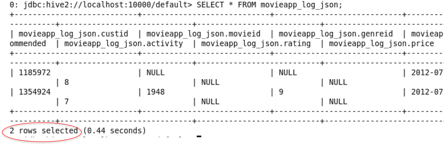
SELECT
* FROM movieapp_log_json;
Result: The Hive table returns the file's only two
records, which look something like this (your two rows
may show different data):
Return to SQL Developer and - without making any
changes to the Oracle table - query movieapp_log_json:
SELECT * FROM
movieapp_log_json;
Result: Oracle Big Data SQL queried the Hive
Metastore and picked up the change in LOCATION.
The Oracle table returns the same two rows (your two
rows will be the same as returned in Hive).
Finally, reset the Hive table and then confirm that
there are more than two rows. Execute the
following commands at the beeline prompt.
ALTER
TABLE movieapp_log_json SET LOCATION
"hdfs://bigdatalite.localdomain:8020/user/oracle/moviework/applog_json";
select
* from movieapp_log_json limit 10;
Note: The query should return 10 rows.
Accessing the recommendation data in Oracle NoSQL
Database will utilize the same method. Return to
SQL Developer and create the recommendation
table. Then, select the first 20 rows from the
table:
CREATE TABLE
RECOMMENDATION
(
CUSTID NUMBER
, SNO NUMBER
, GENREID NUMBER
, MOVIEID NUMBER
)
ORGANIZATION EXTERNAL
(
TYPE ORACLE_HIVE
DEFAULT DIRECTORY DEFAULT_DIR
ACCESS PARAMETERS
(
com.oracle.bigdata.tablename:
moviework.recommendation
)
)
REJECT LIMIT UNLIMITED;
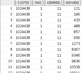
SELECT * FROM recommendation WHERE rownum <=20;
Result: Oracle Big Data SQL queried the Hive
Metastore to determine how to access the Oracle NoSQL
Database table. It then used that information to
retrieve the first 20 rows from the key-value store:
Part 4 - Big Data SQL Performance Features
Big Data SQL provides numerous features that enhance query
performance. These include:
SmartScan: data local scans on the Hadoop cluster that
will filter data based on SQL query predicates
Storage Indexes: automatically generated, in-memory
indexes that enable SmartScan to skip reading blocks that do
not contain data based on the query predicate
Bloom Filters: pushes a predicate that was applied to
a joined look-up table to the data stored on the hadoop
cluster
Partition Pruning: avoid reading hive partitions based
on query predicates
Predicate Pushdown: intelligent data sources - like
Oracle NoSQL Database, HBase, Parquet and ORC files - are able
to process predicates and leverage optimized storage
performance capabilities.
Using a simple, single-node VM is not an environment for
evaluating performance. However, Big Data Lite will allow
you to utilize Partition Pruning and Predicate Pushdown -
enabling you to better understand how these performance features
work. Because Big Data Lite does not include Big Data SQL
Cells, you will not be able see the value from SmartScan,
Storage Indexes and Bloom Filter features.
Querying Partitioned Hive Tables
In this exercise, we will examine the performance impact
of Hive partition pruning. The hive table movieapp_log_avro
is a non-partitioned table defined over Avro
data; we queried this table in a previous exercise.
A second table has been created - movieapp_log_month_avro
- that is partitioned by month.
Launch beeline and review table definition and its
partitions
In SQL Developer, create a Big Data SQL-enabled table
over the hive partitioned table
Compare query performance between the non-partitioned
and partitioned sources
In beeline, review the definition and partitions for
table movieapp_log_month_avro:
Note, this is the same data found in the
non-partitioned hive table. It is simply divided
into 4 partitions.
In SQL Developer, create a Big Data SQL-enabled table
over the partitioned hive table. Notice, you do
not have to specify anything about the partition
definition. Oracle Database queries the hive
metastore at query compilation time to determine the
partitions:
CREATE TABLE
MOVIEAPP_LOG_MONTH_AVRO
(
CUSTID NUMBER
, MOVIEID NUMBER
, ACTIVITY NUMBER
, GENREID NUMBER
, RECOMMENDED VARCHAR2(4)
, TIME VARCHAR2(20)
, RATING NUMBER
, PRICE NUMBER
, POSITION NUMBER
, MONTH VARCHAR2(8)
)
ORGANIZATION EXTERNAL
(
TYPE ORACLE_HIVE
DEFAULT DIRECTORY DEFAULT_DIR
ACCESS PARAMETERS
(
com.oracle.bigdata.tablename:
default.movieapp_log_month_avro
)
)
REJECT LIMIT UNLIMITED;
Query the non-partitioned and partitioned sources and
notice the performance difference:
-- non-partitioned
SELECT movieid,
COUNT(*)
FROM mylogdata
WHERE SUBSTR(TIME, 1, 7) = '2012-07'
AND
movieid
= 11547
GROUP BY movieid;
Result: The query output looks similar to the
following:
   MOVIEID   COUNT(*)

                          ---------- ----------


                          11547       1716


                          Elapsed: 00:00:11.561
-- partitioned
SELECT movieid,
COUNT(*)
FROM movieapp_log_month_avro
WHERE MONTH = '2012-07'
AND movieid = 11547
GROUP BY movieid;
   MOVIEID   COUNT(*)

                            ---------- ----------


                            11547       1716


                            Elapsed: 00:00:03.611
Notes:
Due to partition pruning, the query over the
partitioned source is scanning approximately
one-fourth data. As a result, the query
performance is approximately four times faster.
When running a real Hadoop cluster with Big Data
SQL Server cells, SmartScan and Storage Indexes
would engage to enhance performance.
Predicate Pushdown to Intelligent
Sources
A delimited text file is not an intelligent data
source. The data contained in the source may be
interesting - but there it doesn't provide capabilities to
optimize retrieval of data. Oracle NoSQL Database,
Parquet and ORC files are examples are intelligent
sources. They provide numerous features that
optimize data retrieval. You can review this
blog post for details.
This exercise will examine the performance benefit of
predicate pushdown into Parquet files - which provides a
compressed, efficient columnar store. This example
uses the same data as found in the previous example;
movieapp_log_month_parquet is a partitioned
hive table where data for each month is stored in Parquet
format.
Launch beeline and review the table definition and
its partitions
In SQL Developer, create a Big Data SQL-enabled table
over the hive partitioned table
Compare query performance between the parquet source
and the previous example
In beeline, review the definition and partitions for
table movieapp_log_month_parquet:
Note, this data is the same as the Avro example above
- but in Parquet format.
In SQL Developer, create a Big Data SQL-enabled table
over the partitioned hive table. Notice, you do
not have to specify anything about the partition
definition. Oracle Database queries the hive
metastore at query compilation time to determine the
partitions:
CREATE TABLE
MOVIEAPP_LOG_MONTH_PARQUET
(
CUSTID NUMBER
, MOVIEID NUMBER
, ACTIVITY NUMBER
, GENREID NUMBER
, RECOMMENDED VARCHAR2(4)
, TIME VARCHAR2(20)
, RATING NUMBER
, PRICE NUMBER
, POSITION NUMBER
, MONTH VARCHAR2(8)
)
ORGANIZATION EXTERNAL
(
TYPE ORACLE_HIVE
DEFAULT DIRECTORY DEFAULT_DIR
ACCESS PARAMETERS
(
com.oracle.bigdata.tablename:
default.movieapp_log_month_parquet
)
)
REJECT LIMIT UNLIMITED;
Query the non-partitioned and partitioned sources and
notice the performance difference:
-- partitioned parquet table
SELECT movieid,
COUNT(*)
FROM movieapp_log_month_parquet
WHERE MONTH = '2012-07'
AND movieid = 11547
GROUP BY movieid;
   MOVIEID   COUNT(*)

                            ---------- ----------


                            11547       1716


                            Elapsed: 00:00:00.532
Notes:
Query performance benefits are cumulative.
In this example, the query benefits from both
partition pruning and the Parquet data source.
The elapsed query time has been significantly
reduced.
Part 5 - Applying Oracle Database Security Policies Across
the Big Data Platform
In most deployments, the Oracle Database contains critical and
sensitive data that must be protected. A rich set of
Oracle Database security features, including strong
authentication, row level access, data redaction, data masking,
auditing and more - have been utilized to ensure that data
remains safe. These same security policies can be
leveraged when using Oracle Big Data SQL. This means that
a single set of security policies can be utilized to protect all
of your data.
In our example, we need to protect personally identifiable
information, including the customer last name and customer
id. To accomplish this task, an Oracle Data Redaction
policy has already been set up on the customer
table that obscures these two fields. This was accomplished by
using the DBMS_REDACT PL/SQL package, shown here:
The first PL/SQL call creates a policy called customer_redaction:
It is applied to the cust_id column moviedemo.customer
table
It performs a partial redaction - i.e. it is not nec.
applied to all characters in the field
It replaces the first 7 characters with the number "9"
The redaction policy will always apply - since the
expression describing when it will apply is specified as "1=1"
The second API call updates the customer_redaction
policy, redacting a second column in that same table. It
will replace the characters 3 to 25 in the LAST_NAME
column with an '*'. Note: the application of redaction
policies does not change underlying data. Oracle Database
performs the redaction at execution time, just before the data
is displayed to the application user.
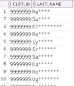
Querying these two columns in the customer table produces the
following result:
SELECT cust_id, last_name FROM
customer;
Importantly, SQL executed against redacted data remains
unchanged. For example, queries can use the cust_id and
last_name columns in join conditions, apply filters to them,
etc. The fact that the data is redacted is transparent to
application code.
In the next section, you apply redaction policies to our tables
that have data sourced in Hadoop.
Apply Redaction Policies to Data
Stored in Hadoop and Oracle NoSQL Database
Here, you apply an equivalent redaction policy to two of
our Oracle Big Data SQL tables, with the following
effects:
The first procedure redacts data sourced from JSON in
HDFS
The second procedure redacts Avro data sourced from
Hive
The third procedure redacts data sourced from Oracle
NoSQL Database
Both policies redact the custid;
attribute.
Go to the SQL Developer Worksheet and run the
following two PL/SQL DBMS_REDACT.ADD_POLICY
procedures:
Result: As stated previously, the custid
column for the three objects are now redacted.
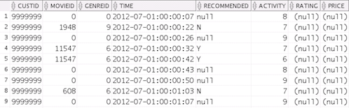
Review the redacted data from the Avro source:
SELECT * FROM mylogdata
WHERE rownum < 20;
Result: The output should look like this:
Notice how the custid column displays a
series of 9s instead of the original value.
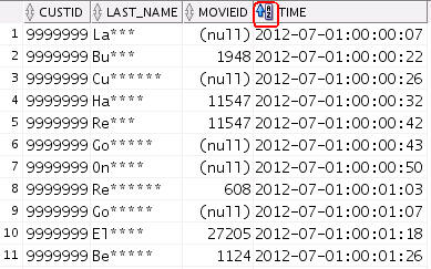
Join the redacted HDFS data to the customer
table by executing the following SELECT statement:
SELECT f.custid,
c.last_name, f.movieid, f.time
FROM customer c, movielog_v f
WHERE c.cust_id = f.custid;
Results: The query output looks similar to the
following:
Notes:
As highlighted in the example above, we used the Sort
tool in the TIME column to sort the output in
ascending order by TIME.
As you can see, the redacted data sourced from
Hadoop works seamlessly with the rest of the data in
your Oracle Database.
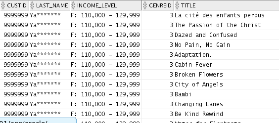
Similarly, join the redacted NoSQL data to the customer
and movie Oracle Database tables by
executing the following SELECT statement:
SELECT f.custid,
c.last_name, c.income_level, f.genreid, m.title
FROM customer c, recommendation f, movie m
WHERE c.cust_id = f.custid
AND f.movieid = m.movie_id
AND c.income_level like 'F%'
ORDER BY f.custid, f.genreid;
Results: The query output displays recommendations
for wealthier customers:
Notes:
You can now easily see movies that are recommended
to customers - while preserving sensitive, customer
identity.
Part 6 - Using Oracle Analytic SQL Across All Your Data
Oracle Big Data SQL allows you to utilize Oracle's rich SQL
dialect to query all your data, regardless of where that data
may reside. We will take a look at a couple of analytic
queries that deliver unique insights across our three data
sources.
Gaining Insights From All Your
Data
This next example will enrich Oracle MoviePlex's
understanding of customers by utilizing an RFM analysis.
This query will identify:
Recency : when was the last time the customer accessed
the site?
Frequency : what is the level of activity for that
customer on the site?
Monetary : how much money has the customer spent?
To answer these questions, SQL Analytic Functions will be
applied to data residing in both the application logs on
Hadoop and sales data in Oracle Database tables. Customers
will be categorized into 5 buckets measured in increasing
importance. For example, an RFM combined score of 551
indicates that the customer is in the highest tier of
customers in terms of recent visits (R=5) and activity on
the site (F=5), however the customer is in the lowest tier
in terms of spend (M=1). Perhaps this is a customer that
performs research on the site, but then decides to buy
movies elsewhere!
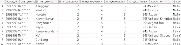
We want to target customers who we may be losing to
competition. Therefore, execute the following query
-- which finds important customers (high monetary score)
that have not visited the site recently (low recency
score):
Go to the SQL Developer Worksheet and run the
following query:
WITH
customer_sales AS (
-- Sales and customer attributes
SELECT m.cust_id,
c.last_name,
c.first_name,
c.country,
c.gender,
c.age,
c.income_level,
NTILE (5) over (order by sum(sales)) AS rfm_monetary
FROM movie_sales m, customer c
WHERE c.cust_id = m.cust_id
GROUP BY
m.cust_id,
c.last_name,
c.first_name,
c.country,
c.gender,
c.age,
c.income_level
),
click_data AS (
-- clicks from application log
SELECT custid,
NTILE (5) over
(order by max(time)) AS rfm_recency,
NTILE (5) over
(order by count(1)) AS
rfm_frequency
FROM movielog_v
GROUP BY custid
)
SELECT c.cust_id,
c.last_name,
c.first_name,
cd.rfm_recency,
cd.rfm_frequency,
c.rfm_monetary,
cd.rfm_recency*100 +
cd.rfm_frequency*10 + c.rfm_monetary AS
rfm_combined,
c.country,
c.gender,
c.age,
c.income_level
FROM customer_sales c, click_data cd
WHERE c.cust_id = cd.custid
AND c.rfm_monetary >= 4
AND cd.rfm_recency <= 2
ORDER BY c.rfm_monetary desc, cd.rfm_recency
desc;
Notes:
The customer_sales subquery selects
from the Oracle Database fact table
movie_sales to categorize customers based
on sales.
The click_data subquery performs a
similar task for web site activity stored in the
application logs - categorizing customers based on
their activity and recent visits.
These two subqueries are then joined to produce
the complete RFM score. The result only shows
customers who have significant spend (>= 4) but
have not visited the site recently (<= 2).
Result: The query output looks similar to the
following:
These are the at-risk customers for Oracle MoviePlex.
They were at one time active, big spenders on the site.
Let's see what we can do to bring them back!
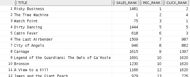
How is the recommendation engine performing? To
answer this question, we will need to understand the
following:
Rank how many times movies are recommended (from
Oracle NoSQL Database)
Rank sales revenue for movies (from Oracle
Database tables)
Rank interest level in a movie - i.e. how many
times people have previewed, watched, displayed more
info, etc. (from HDFS click data)
WITH rank_recs AS (
-- recommendation rank from NoSQL Database
SELECT movieid,
RANK
() OVER (ORDER BY COUNT(movieid) DESC) AS rec_rank
FROM recommendation
GROUP BY movieid),
rank_sales AS (
-- sales rank from Oracle Database
SELECT m.movie_id,
m.title,
RANK
() OVER (ORDER BY SUM(ms.sales) DESC) as sales_rank
FROM movie m, movie_sales ms
WHERE ms.movie_id = m.movie_id
GROUP BY m.title, m.movie_id
),
rank_interest AS (
-- "interest" rank from hdfs logs
SELECT movieid,
RANK () OVER (ORDER BY COUNT(movieid) DESC) AS
click_rank
FROM movielog_v
WHERE activity IN (1,4,5) -- rated, started or
browsed the movie
GROUP BY movieid
)
-- combine the results
SELECT rs.title,
sales_rank,
rec_rank,
click_rank
FROM rank_recs rr, rank_sales rs, rank_interest ri
WHERE rr.movieid = rs.movie_id
AND ri.movieid = rs.movie_id
ORDER BY rec_rank asc;
Result: The query output looks like this:
Notes:
By combining
results from all three data sources, we are able to
get a complete view of the customer activity.
Part 7 - Introduction to SQL Pattern Matching
This section covers the new SQL pattern matching and analytical
SQL functionality that is part of Oracle Database 12c.
Row pattern matching in native SQL improves application
development, developer productivity and query efficiency for
row-sequence analysis. This new feature is an important addition
to your SQL toolbox.
Introduction
Recognizing patterns in a sequence of rows has been a
capability that was widely desired, but not really possible with
SQL until now. There were many workarounds, but these were
difficult to write, hard to understand, and inefficient to
execute. With Oracle Database 12c you can use the MATCH_RECOGNIZE
clause to perform pattern matching in SQL to do the following:
Logically group and order the data that is used in the MATCH_RECOGNIZE
clause using the PARTITION
BY and ORDER BY clauses.
Define business rules/patterns using the PATTERN
clause. These patterns use regular expressions syntax, a
powerful and expressive feature and applied to the pattern
variables.
Specify the logical conditions required to map a row to a
row pattern variable using the DEFINE
clause.
Define output measures, which are expressions within the MEASURES
clause.
Control the output (summary vs. detailed) from the pattern
matching process
The moviedemo schema contains a view called MOVIEAPP_LOG_JSON_V
which returns a formatted version of JSON click data stream from
our web application log file. The view returns the following
columns:
Using this click data we will create a sessionization data set
which tracks each session, the duration of the session and the
number of clicks/events.
Tasks and Keywords in Pattern
Matching
Let us go over some of the tasks and keywords used in
pattern matching. Building a pattern matching statement
can be broken down into four simple steps:
Task
Keyword
Description
1. Organize the data
PARTITION
BY
ORDER BY
Logically divide/partition the rows into groups
Logically order the rows within a partition
2. Define the business rules
PATTERN
DEFINE
AFTER MATCH
Defines the pattern variables that must be
matched, the sequence in which they must be matched,
and the number of rows which must be matched
Specifies the conditions that define a pattern
variable
Determines where to restart the matching process
after a match is found
3. Define the output measures
MEASURES
MATCH_NUMBER
CLASSIFIER
Defines row pattern measure columns
Finds which pattern variable applies to which rows
Identifies which component of a pattern applies to a
specific row
4. Control the output
ONE
ROW PER MATCH
ALL ROWS PER MATCH
Returns one summary row of output for each match
Returns one detail row of output for each row of
each match
Pattern Match Example: Web Log
Sessionization Analysis
Defining the pattern/business rules
For this scenario we are going to assume that a
series of events or clicks within our web log file are
part of the same session if the date-time between
events (clicks) is less than 2 hours (when people
are watching a movie they are not recording any
click activity so if we set this threshold too low
we run the risk of splitting up single sessions into
multiple sessions). The exact definition of a
session will need to come from the business users and
of course using SQL pattern matching it is relatively
simple to change the session threshold to say two
minutes if that was the specific requirement from the
business.
Using this information we can now build our PATTERN
and DEFINE
clauses.
the plus sign (+) indicates that we are looking for
at least one or more instances of our pattern, i.e.
each event must fall within a two hour boundary of the
PREVIOUS event which is captured by the element
sess.time_id.
To capture this information we are using one of many
built-in functions that allows us to point to specific
values within the dataset as it is being processed (there
is more information about this later in this lab
There are many other regular expressions that we can
use and these are all discussed in the Data
Warehouse Guide.
Using built-in functions
The MATCH_RECOGNIZE
feature comes with some very useful built-in functions
that you can include in your code:
MATCH_NUMBER:
You might have a large number of matches for your
pattern inside a given row partition. How do you
tell all these matches apart? This is done with the
MATCH_NUMBER
function. Matches within a row pattern partition are
numbered sequentially starting with 1 in the order
they are found. Note that match numbering starts
over again at 1 in each row pattern partition,
because there is no inherent ordering between row
pattern partitions.
CLASSIFIER:
Along with knowing which MATCH_NUMBER
you are seeing, you may want to know which component
of a pattern applies to a specific row. This is done
using the CLASSIFIER
function. The classifier of a row is the pattern
variable that the row is mapped to by a row pattern
match. The function returns a character string whose
value is the classifier of a row. The classifier of
a row that is not mapped by a row pattern match is
null.
Once we have identified a group of records as
belonging to a unique session we need a way to
identify each unique session within our resultset. To
do this we can use the built-in measure MATCH_NUMBER()
to apply a sequential number to each of our unqiue
sessions. At the same time we will use the CLASSIFIER()
function to show which pattern variable is matched for
each row. Using this information we can build our MEASURE
clause:
MEASURES
MATCH_NUMBER() session_id,
CLASSIFIER()
AS pattern_id,
Detailed or summary report?
For this first step in creating our sessionization
data set we will return a detailed report by using the
ALL ROWS PER
MATCH syntax.
Returning a simple sessionization result set
We can now bring all of the above information
together and build our pattern matching statement.
This simple SELECT statement returns the session id
from our MATCH_RECOGNIZE clause along with all the
columns from our source view. As part of this example
we have used a final WHERE
clause to restrict the output rows to one specific
customer (1000693):
SELECT *
FROM movieapp_log_json_v
MATCH_RECOGNIZE
(PARTITION BY cust_id ORDER BY time_id
MEASURES MATCH_NUMBER() AS
session_id
ALL ROWS PER MATCH
PATTERN (bgn sess+)
DEFINE
sess
as time_id <= PREV(sess.time_id) + interval '2'
hour
)
WHERE cust_id ='1000693';
The output from this MATCH_RECOGNIZE statement should
look something like this:
Our automatic calculation to determine the session id
is shown in column 3. Now we have successfully
converted our original web log file into a basic
sessionization data set. Note that that we could now
share this data set with our business users. But
before we do that we might want to do some more work
to make sure our pattern matching process is working
correctly.
Part 8 - Checking the Pattern Matching Process
In this section, we will use the CLASSIFIER()
measure to show which pattern variable is being assigned to each
row. This will help us debug our pattern matching process and
ensure it is working correctly.
Adding CLASSIFIER measure
We need to expand the MEASURE clause and include the built-in
function CLASSIFIER().
MEASURES
MATCH_NUMBER() AS session_id,
CLASSIFIER()
AS pattern_id
Selecting specific columns
We are going to amend the SELECT
clause to only return the customer id, session id (from our MATCH_NUMBER()
function), date, time and the pattern id (from our CLASSIFIER()
function). The new code should look like this:
SELECT
cust_id,
session_id,
time_id,
TO_CHAR(time_id, 'hh24:mi:ss') AS
session_time,
pattern_id
FROM movieapp_log_json_v
MATCH_RECOGNIZE
(PARTITION BY cust_id ORDER BY time_id
MEASURES MATCH_NUMBER() AS session_id,
CLASSIFIER()
AS pattern_id
ALL ROWS PER MATCH
PATTERN (bgn sess+)
DEFINE
sess
as time_id <= PREV(sess.time_id) + interval '2' hour
)
WHERE cust_id ='1000693';
The output from this MATCH_RECOGNIZE
statement should look something like this:
We can see that each new session starts with the BGN
pattern and then all other clicks are within a 2 hour window
of their previous SESS.time
event and are marked with the pattern SESS.
Now we have a much better data set for our business users
but we can still make improvements to the data set.
Part 9 - Creating a More Useful Data Set
Using the CLASSIFIER()
function we have established that our pattern matching process
is working correctly. What we need to do now is condense the
data set so that we have one row for each session. We can do
that by changing the way we output the data. It would be also
useful to include some additional business metrics as part of
the of the data set. The following sections will explain how to
do this.
Creating a Summary Report
Using ONE ROW
PER MATCH
We need to change the output clause from ALL
ROWS PER MATCH to ONE
ROW PER MATCH.
Updating the measure clause
As we are now creating a summary report we need to
remove the CLASSIFIER()
function from the MEASURE
clause.
Selecting specific columns
We are going to amend the SELECT
clause to return only the customer id and session id
(from our MATCH_NUMBER()
function) for the this summary report. The new code
should look like this:
SELECT cust_id,
session_id
FROM movieapp_log_json_v
MATCH_RECOGNIZE
(PARTITION BY cust_id ORDER BY time_id
MEASURES MATCH_NUMBER() AS
session_id ONE ROW PER MATCH
PATTERN (bgn sess+)
DEFINE
sess
as time_id <= PREV(sess.time_id) + interval '2'
hour
)
WHERE cust_id ='1000693';
The output from this MATCH_RECOGNIZE statement should
look something like this:
The report should have 31 rows. The report now shows
one row per session. However, this information is not
especially useful for our business users. We can add
more useful information to this report by expanding
the measure clause.
Adding Business Value
Calculating the number of clicks in a session
We can return a count of the number of clicks within
a session by using the COUNT()
function within the MEASURE
clause.
MEASURES MATCH_NUMBER() AS
session_id, COUNT(*)
AS no_of_events
Finding the start and end time of a session
We can find the start time and end time of session by
using one of the unique features of MATCH_REOGNIZE
- the ability to point to specific values within a
column by referencing the relevant pattern
expressions. MATCH_RECOGNIZE
includes some additional functions that help us
extract a data points within a specific column. These
new functions include:
FIRST
LAST
NEXT
PREVIOUS
Updated measure clause
Using these new functions we can now expand the
measure clause to return the start time and end time
of each session.
MEASURES
MATCH_NUMBER() AS session_id,
COUNT(*)
AS no_of_events, TO_CHAR(FIRST(bgn.time_id),'hh24:mi:ss')
AS start_time,
TO_CHAR(LAST(sess.time_id),'hh24:mi:ss')
AS end_time
Calculating the duration of a session
We can calculate the duration of session by taking the
start time of each session from the end time of each
session. To do that we can use the normal database
date-time functionality.
MEASURES MATCH_NUMBER() AS
session_id,
COUNT(*)
AS no_of_events,
TO_CHAR(FIRST(bgn.time_id),'hh24:mi:ss')
AS start_time,
TO_CHAR(LAST(sess.time_id),'hh24:mi:ss')
AS end_time, TO_CHAR(to_date('00:00:00','HH24:MI:SS')
+
(LAST(sess.time_id)-FIRST(bgn.time_id)),'hh24:mi:ss')
AS mins_duration
SQL to generate summary report
Our revised SQL statement now looks like this:
SELECT
cust_id,
session_id, no_of_events,
start_time,
end_time,
mins_duration
FROM movieapp_log_json_v
MATCH_RECOGNIZE
(PARTITION BY cust_id ORDER BY time_id
MEASURES MATCH_NUMBER() AS
session_id, COUNT(*)
AS no_of_events,
TO_CHAR(FIRST(bgn.time_id),'hh24:mi:ss')
AS start_time,
TO_CHAR(LAST(sess.time_id),'hh24:mi:ss')
AS end_time,
TO_CHAR(to_date('00:00:00','HH24:MI:SS')
+
(LAST(sess.time_id)-FIRST(bgn.time_id)),'hh24:mi:ss')
AS mins_duration
ONE ROW PER MATCH
PATTERN (bgn sess+)
DEFINE
sess
as time_id <= PREV(sess.time_id) + interval '2'
hour
)
WHERE cust_id ='1000693';
The output from this MATCH_RECOGNIZE statement should
look something like this:
Our new summary report now shows one row per session
and we have add more a lot of useful information for
our business users by expanding the measure clause to
show the start time, end time and duration of each
session. This gives our business users a great place
to start their analysis.
Part 10 - Other Useful 12c Analytical SQL Features
To make the following code easier to read we have wrapped the MATCH_RECOGNIZE
clause that we created above within a view called movieapp_analytics_v.
Of course you could incorporate the following additional
features into the MATCH_RECOGNIZE
statements above.
How Many Distinct Customers?
A useful metric within click data is to count the number
of distinct customers using our site each month. Normally
we would just use the COUNT(DISTINCT
expr) function. However, this can require a lot
of resources to search through a large dataset and return
the exact number of distinct values.
With the release of Database 12c Oracle provides a much
faster way to do this type of analysis. Using APPROX_COUNT_DISTINCT
it is possible to get a reasonably accurate estimate of
the number of distinct values within a column. This new
function can process large amounts of data significantly
faster than COUNT(DISTINCT
expr) function, with negligible deviation from
the exact result. For more information about this new
feature please refer to the SQL
Reference Guide
Let's calculate the number of unique sessions per month
using both functions:
Using APPROX_COUNT_DISTINCT
Add new function to SELECT
statement and for comparison purposes also include COUNT(DISTINCT...)
function:
SELECT
time_id,
SUM(no_of_events) AS tot_events, COUNT(DISTINCT cust_id) AS
unique_customers,
APPROX_COUNT_DISTINCT(cust_id) AS
est_unique_customers
FROM movieapp_analytics_v
GROUP BY time_id
ORDER BY 1;
The output from this statement should look like this:
The report shows the number of distinct customers per
month and the approximate number of distinct customers
per month. This type of summary report is usually the
basis for doing for further analysis, i.e. if the
counts are significantly higher or lower then further
analysis might be required. Therefore, using the new APPROX_COUNT_DISTINCT
function means our business users can get their
results much faster without having to sacrifice too
much in terms of accuracy
Finding the Top 1% of Customers
Another useful metric within click data is finding
out who are our best customers and worst. Using the
new Top-N
syntax we can very quickly find the top 1% of our
customers based on total number sessions and the
number of clicks they recorded
The new syntax for TOP-N support was introduced in
12c and is shown here:
This new function can process large amounts of data
significantly faster than COUNT(DISTINCT
expr) function, with negligible deviation from
the exact result. For more information about this new
function please refer to the SQL
Reference Guide
Top N SQL code
Using our new FETCH
syntax we can easily find our top 1% customers:
SELECT
cust_id,
MAX(session_id) AS no_of_sessions, SUM(no_of_events) AS
tot_clicks_session,
TRUNC(AVG(no_of_events)) AS
avg_clicks_session,
MIN(no_of_events) AS
min_clicks_session
MAX(no_of_events) AS
max_clicks_session
FROM movieapp_analytics_v
GROUP BY cust_id
ORDER BY 2 DESC, 3 DESC FETCH FIRST 1 PERCENT ROWS ONLY;
For more information about this new feature please refer
to the SQL
Reference Guide
The output from this statement should look something
like this:
The report shows our top 1% customers based on number
of sessions and number of clicks recorded during a
session and it contains 23 rows.
Finding the Bottom 1% of
Customers
Bottom N SQL code
To find the bottom 1% of customers we simply need to
reverse the sort order!
SELECT
cust_id,
MAX(session_id) AS no_of_sessions,
SUM(no_of_events) AS tot_clicks_session,
TRUNC(AVG(no_of_events)) AS
avg_clicks_session,
MIN(no_of_events) AS min_clicks_session,
MAX(no_of_events) AS max_clicks_session
FROM movieapp_analytics_v
GROUP BY cust_id
ORDER BY 2 ASC, 3 ASC FETCH FIRST 1 PERCENT ROWS ONLY;
Summary
In this tutorial, you have learned how to:
Configure Oracle Big Data SQL on Oracle Exadata
Create Oracle external tables that access data in HDFS,
Oracle NoSQL Database and Hive
Apply Oracle security policies across data in both Oracle
Database and Hadoop
Use Oracle's rich SQL dialect to analyze data across the
data platform
Use Oracle's new rich SQL pattern matching features to
analyze web log data
Use the MATCH_RECOGNIZE
clause to perform pattern matching in SQL
Use the main keywords that are used in pattern matching
Create sessionization analysis from web log file data
Quickly change the business rules for an existing query
Add calculated measures to increase business value
Speed up processing by using the new APPROX_COUNT_DISTINCT
function to quickly calculate number of distinct values
Quickly find the top/bottom values using the new FETCH
feature
For detailed information on pattern matching, see the Pattern
Matching chapter in the Oracle
Database 12c Data Warehousing Guide reference
guide. Among other things, this chapter contains the following
detailed examples:
Stock Market Examples: based on common
tasks involving share prices and patterns.
Security Log Analysis Examples: deals with
a computer system that issues error messages and
authentication checks, and stores the events in a system file.
Sessionization Examples: analysis of user
activity, typically involving multiple events in a single
session. Pattern matching makes it easy to express queries for
sessionization.