Using Feature Selection and Generation with GLM
Overview
- Feature Selection is the process of selecting the most meaningful attributes. With feature selection, GLMs can be created with fewer predictors, leading to smaller models and faster scoring.
- Feature Generation is the process of combining attributes into new features. With feature generation, GLMs use non-linear terms (up to cubic terms), leading to more powerful models and increased transparency.
- Identify and select two new data sources from the Oracle Database sample SH schema: the SALES and CUSTOMERS tables.
- Summarize the QUANTITY_SOLD and AMOUNT_SOLD measures from the SALES table by Customer and Product, over the Promotion and Channel dimensions.
- Place the summarized data into a new table.
- Join the summarized sales data with customer data to provide a pool of data for the Classification model.
- Apply the Feature Selection / Generation option with a GLM algorithm and examine the results.
- Have access to or have installed:
- Oracle Database 12c Enterprise Edition, Release 12.1 with Advanced Analytics Option.
- The Oracle Database sample data, including the unlocked SH schema.
- SQL Developer 4.0
- Set up Oracle Data Miner for use within Oracle SQL Developer 4.0. If you have not already set up Oracle Data Miner, complete the lesson: Setting Up Oracle Data Miner 4.0
- Completed the lesson: Using Oracle Data Miner 4.0
Purpose
This tutorial covers the use of Oracle Data Miner 4.0 to leverage enhancements to the Oracle implementation of Generalized Liner Models (GLM) for Oracle Database 12c. These enhancements include support for Feature Selection and Generation. In this lesson, you learn how to use these GLM enhancements in a Classification model.
Time to Complete
Approximately 30 mins.
Introduction
Generalized Linear Models provide great transparency, which may be achieved at the expense of accuracy. With the introduction of a feature selection and generation capability, GLMs can maintain a high degree of accuracy without sacrificing transparency (the ability to explain the predictions made by the model).
In this lesson, you will create a new workflow that illustrates these enhancements.
Scenario
This lesson focuses on a business problem that can be solved by applying a Classification model. In our scenario, ABC Company wants to know which customer attributes are most significant in predicting the gender of a customer. The new feature selection / generation enhancements are used as part of this mining exercise.
In this new workflow, you:
The completed workflow looks like this:

Software Requirements
The following is a list of software requirements:
Prerequisites
Before starting this tutorial, you should have:
Create a Data Miner Project
Here, you will create a new project using the same techniques shown in the "Using Oracle Data Miner 4.0" tutorial.
NOTE: If you have already completed the lesson Using the SQL Query Node in a Workflow, skip this topic and go to Build the Data Miner Workflow.
To create a Data Miner Project, perform the following steps:
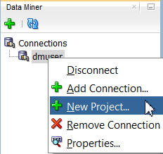
In the Data Miner tab, right-click dmuser and select New Project, as shown here:
In the Create Project window, enter a project name (in this example SH Schema) and then click OK.
Note: You may optionally enter a comment that describes the intentions for this project. This description can be modified at any time.
Result: The new project appears below the data mining user connection node.
Note: In this image, the project that was created in the "Using Oracle Data Miner 4.0" tutorial is also shown.
Build the Data Miner Workflow
- Identify and combine data from multiple data sources
- Create three GLM Classification models
- Build and compare model results
- In the middle of the SQL Developer window, an empty workflow canvas opens with the name that you specified.
- On the upper right-hand side of the interface, the Components tab of the Workflow Editor appears.
- If you have completed the lesson Using the SQL Query Node in a Workflow, then you already have access to the SH schema -- skip step 4. and go directly to step 5.
- If you have not completed the lesson Using the SQL Query Node in a Workflow, then continue with step 4.
- Use an Aggregate node to aggregate the AMOUNT_SOLD and QUANTITY_SOLD measures from the SALES table. The measures will be aggregated by Customer and Product, over the Promotion and Channel dimensions.
- Create a table for the aggregated sales data.
- Use a Join node to join the aggregated sales data to the CUSTOMERS table.
- De-select the Auto Input Columns Selection option.
- Select the Index option for the CUST_ID column.
- Click OK.
- Select CUSTOMERS as Source 1, and Create Table as Source 2.
- Select the CUST_ID column from both sources.
- Then, click the Add button to define the Join Columns.
- Deselect the Automatic Settings option.
- Scroll down and select the CUST_ID column from the Create Table node.
- Click the Remove tool (red "x" icon).
- Click Yes in the Warning window.
- Remove all of the default algorithms from the Class Build node except the GLM algorithm.
- Add a second GLM algorithm to the node, and modify it to use the Feature Selection option.
- Add a third GLM algorithm to the node, and modify it to include the Feature Selection and Feature Generation options.
- As seen in the "Using Oracle Data Miner 4.0" lesson, all four classification algorithms are selected by default.
- Next, you will remove the model settings for the SVM, DT, and NB algorithms, and then add a second GLM model setting.
- Therefore, this classification model will be used to predict whether a customer is Male or Female, by using input attributes from the joined source data.
- Although not required, it is advised that you define a Case ID to uniquely define each record. This helps with model repeatability and is consistent with good data mining practices.
- Feature Selection Criteria. Values include System Determined, Akaike Information, Schwarz Bayesian Information, Risk Inflation, and Alpha Investing
- Max Number of Features. You can specify a maximum number or you can let the system determine the value.
- Feature Acceptance. You can select Strict or Relaxed or you can let the system determine which value to apply.
- Prune Model. You can enable or disable this option.
- Categorical Predictor Treatment. Choices include Add One at a Time, or Add All at a Once.
- If you select Add One at a Time, you can also enable Feature Generation, which provides two methods: Quadratic Candidates and Cubic Candidates.
- When the node runs it builds and tests all of the models that are defined in the node.
- As before, a green gear icon appears on the node borders to indicate a server process is running, and the status is shown at the top of the workflow window.
- Viewing the models individually
- Viewing the test results individually, or comparing the test results together
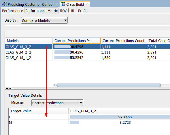
- In the upper pane, the Correct Predictions %, Correct Predictions Count, Total Case Count, and Total Cost is shown for each model.
- For the selected model in the upper pane, target value details are provided in the lower pane.
- Although the correct prediction % and count numbers for the feature selection models are lower than the model that did not use the option, the correct predictions for the target value of Female are just over 97 for the Feature Selection models (GLM_3_2 and GLM_2_2), while the Ridge Regression model (GLM_1_2) shows a correct predictions value of 49 for the target value of Female.
- Select the target value F (for Female)
- De-select the Sort by absolute value option.
- Sort the Coefficient column, in descending order.
- This first model indicates 884 coefficients, ranked by significance, that potentially aid in determining the prediction.
- The most significant attribute is CUST_MARITAL_STATUS. Other attributes are shown in ranked order.
- Recall that this model did not enable feature selection/generation, which is the determining factor in why so many coefficients were selected for this model.
As discussed in the "Using Oracle Data Miner 4.0" tutorial, a Data Miner Workflow is a collection of connected nodes that describe a data mining processes.
Sample Data Mining Scenario
In this topic, you will create a data mining process that identifies which attributes are most significant in predicting the gender of a customer.
To accomplish this goal, you build a workflow that enables you to:
To create the workflow for this process, perform the following steps.
Create a Workflow and Add Data Sources
Right-click your project (SH Schema) and select New Workflow from the menu.
Result: The Create Workflow window appears.
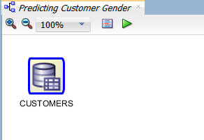
In the Create Workflow window, enter Predicting Customer Gender as the name and click OK.

Result:
The first element of any workflow is the source data. Here, you add the first of two Data Source nodes to the workflow.
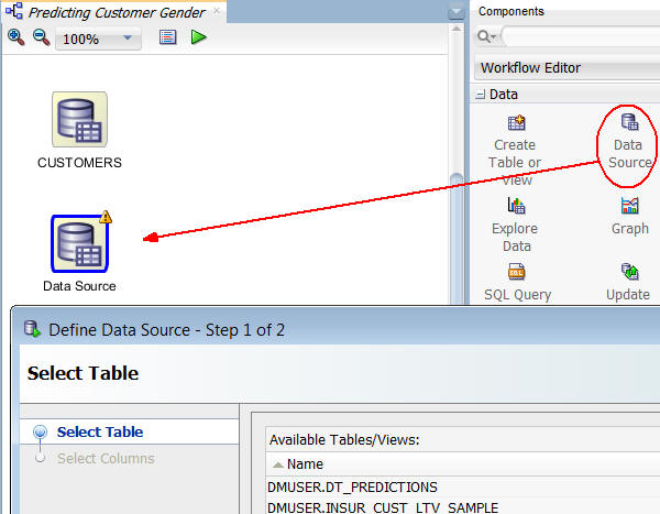
A. In the Components tab, drill on the Data category. A group of six data nodes appear, as shown here:
B. Drag and drop the Data Source node onto the Workflow pane.
Result: A Data Source node appears in the Workflow pane and the Define Data Source wizard opens.
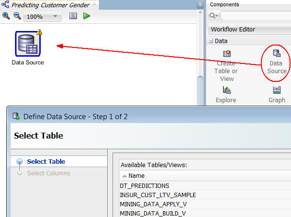
Notes: In the Define Data Source wizard, only tables and views owned by the user are displayed by default. However, for this workflow, you want to use a table in the SH schema.
In Step 1 of the wizard:
A. Click Add Schemas, beneath the Available Tables/Views list, as shown here:
B. In the Edit Schema List window, select SH from the Available Schemas list and move it to the Selected list, as shown below. Then, click OK.
Note: Notice that the Include Tables from Other Schemas option is automatically selected.

Next, scroll down and select the SH.CUSTOMERS table. Then click Finish in the wizard.
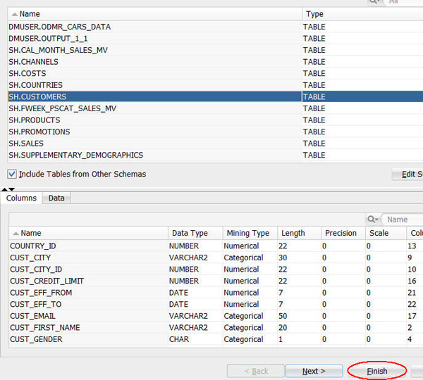
Result: A data source node for the CUSTOMERS table is defined in the workflow.
A. Using the same technique just described, add a second Data Source nodes to the workflow, just underneath the CUSTOMERS data source, like this:
B. In the Define Data Source wizard, select the SH.SALES table and click Finish.

Result: Two data source nodes are now in the Workflow pane, like this:

Aggregate and Join Data
The Transforms node group contains a number of tools that enable you to transform data for use within a workflow. In this topic, you will:
Follow these steps:
In the Components tab, drill on the Transforms group, and then drag and drop the Aggregate node to the Workflow, like this:

Connect the SALES and Aggregate nodes as follows:.
A. Right-click the SALES node and select Connect from the pop-up menu.
B. Drag the pointer to the Aggregate node and click.
Result: the SALES and Aggregate nodes are connected, like this:

Next, use the Aggregate wizard and define the aggregation rules.
A. Double-click the Aggregate node to display the Edit Aggregate Node window. Then, click Edit, as shown here:
B. In the Edit Group By window, move the CUST_ID attribute from the Available list to the Selected list as shown, and then click OK.
C. Next, click the Aggregation Wizard tool, as shown here:

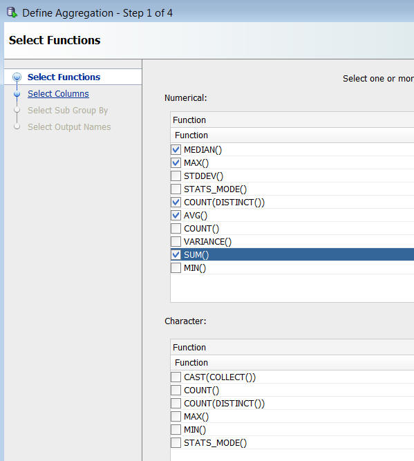
D. In Step 1 of the Define Aggregation wizard, select MEDIAN(), MAX(), COUNT (DISTINCT()), AVG(), and SUM() as the numerical functions, and then click Next.
E. In Step 2 of the wizard, move the AMOUNT_SOLD and QUANTITY_SOLD attributes from the Available list to the Selected list, as shown here. Then click Next.

F. In Step 3 of the wizard, move the PROD_ID attribute from the Available list to the Selected list, as shown here. This identifies Product as the Sub Group By for the aggregations, enabling aggregation by Customer and then by Product.

G. Click Finish in the wizard.
Result: The Edit Aggregation Node window should now look like this (click the Source column to sort as shown):
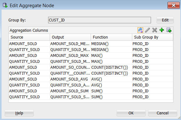
H. Finally, click OK to close the Edit Aggregation Node window.
Result: The yellow "!" icon in the Aggregate node border disappears, signifying that it is ready to use.
Next, you create a table for the aggregated sales data.
A. In the Components tab, open on the Data group and drag a Create Table or View node to the workflow, like this:
B. Connect the Aggregate node to OUTPUT node, and then rename the OUTPUT node to "Create Table". The resulting display should look like this:

Now, create an index on the table to speed up the join.
A. Double-click the Create Table node.
B. In the Edit Create Table or View Node window, perform the following:

Finally, join the table of aggregated sales data to the CUSTOMERS table.
A. From the Transforms group, drag and drop a Join node to the workflow, like this:
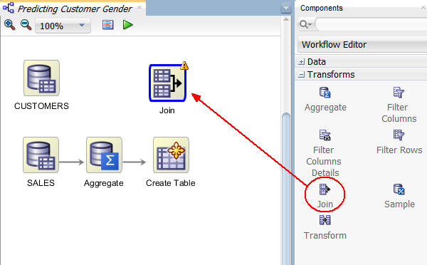
B. Connect the Create Table node to Join node, and the CUSTOMERS node to the Join node, like this:

C. Next, double-click the Join node to display the Edit Join Node window. The Join tab is displayed by default. Then, click the Add (green "+" icon), like this:
D. In the Edit Join Column window:
The Edit Join Column window should look like this:

E. Click OK in the Edit Join Column window.
F. Then, select the Columns tab of the Edit Join Node window, and remove the CUST_ID column from the Create Table source by performing the following:
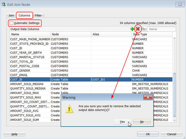
Result: Now, only the CUST_ID column from the CUSTOMERS table is displayed as an output data column, and the total number of specified columns is 33.
G. Finally, click OK in the Edit Join Node window.
The workflow should now look like this:

Create Classification Models
Next, you will add a Classification node to the workflow, like you did in the Using Oracle Data Miner 4.0 tutorial.
However, in this scenario, you will:
Then, in the next topic, you will build the classification models and compare the results of the three GLM models.
Follow these steps:
A. First, expand the Models category in the Components tab, and add a Classification node to the Workflow pane, like this:
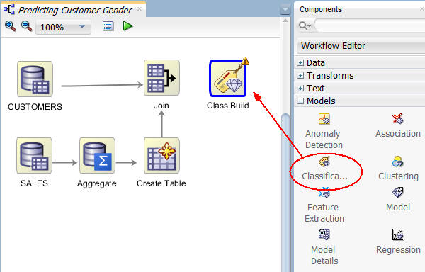
B. Then, connect the Join node to the Class Build node. When the connection is made, the Edit Classification Build node window appears automatically.
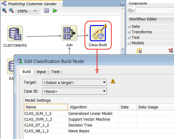
Notes:
Select all of the model settings except for GLM, and then click the Remove tool (red "x" icon), as shown below. (Select Yes in the warning message window.)
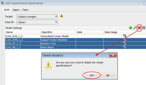
Result: Only the GLM algorithm model setting remains in the list.
In the Edit Classification Build Node window:
A. Select CUST_GENDER as the Target attribute.
B. Select CUST_ID as the Case ID attribute.

Notes:
Next, with the GLM model setting selected, click the Duplicate Selected Model tool, as shown here:
Result: An exact copy of the first GLM model is created, with a new name. (The model name you get may be different.)

Next, you view the default settings for the GLM models, and then modify the duplicated model to add Feature Extraction.
A. With the duplicated model selected (CLAS_GLM_2_2 in this example), click the Edit Advanced Model Settings tool (pencil icon).
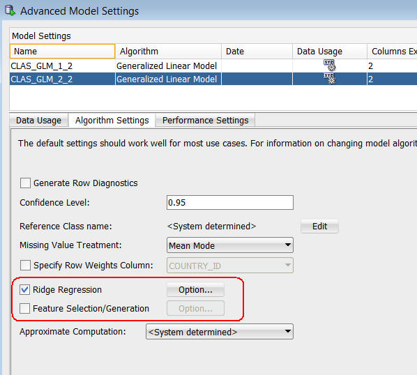
B. In the Advanced Model Settings window, select the Algorithm Settings tab. Notice that Ridge Regression is selected by default, and not Feature Selection/Generation.
C. Select the first GLM model in the list at the top (CLAS_GLM_1_2 in this example), and you will see the same default algorithm settings apply to both models.
Once again, select the second GLM model in the list, select the Feature Selection/Generation option, and then click the associated Option button, as shown here:
In the Feature Selection Option Dialog, we see the default Feature Selection options. Other options include:
However, notice that Feature Generation is not selected by default.
Click OK to save the Feature Selection option without Feature Generation. Then, click OK in the Advanced Model Settings window.
Back in the Edit Classification Build Node window, select the modified GLM model and click the Duplicate Selected Model tool, as shown here.

Result: A third GLM model appears in the list.
Next, select the new GLM model and click the (CLAS_GLM_3_2 in this example), click the Edit Advanced Model Settings tool (pencil icon).
A. In the Algorithm Settings tab of the Advanced Model Settings window, click the Option button next to Feature Selection/Generation, as shown here:

B. In the Feature Selection Option Dialog, select the Feature Generation option, as shown here, and then click OK.

A. To save your change, click OK in the Advanced Model Settings window.
B. Then, click OK in the Edit Classification Build Node window,as shown here:
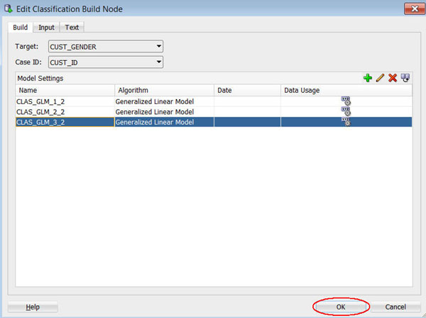
Result: The workflow should now look like this:
Build and Compare the Models
In this topic, you build the three GLM models against the joined source data. Then, you examine the model results. As stated before, we are interested in those input attributes (features) that are most significant in predicting the outcome of customer gender.
In this scenario, we will compare the results of the first GLM model that uses Ridge Regression, to the other two GLM models. The second model uses Feature Selection, and the third model uses both Feature Selection and Feature Generation. We want to see which model produces the highest degree of predictive accuracy without sacrificing transparency.
Right-click the classification build node and select Run from the pop-up menu.
Notes:
When the build is complete, all nodes contain a green check mark in the node border.

Once the build process is complete, you can compare models by:
Right-click the Class Build node and select Compare Test Results from the menu, like this:

Results: A Class Build window opens, showing a graphical comparison of the three models in the Performance tab, as shown here:
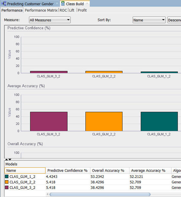
Note: The model results show that the Feature Selection/Generation models produce a slightly higher degree of Predictive Confidence % and Average Accuracy % than model that did not use the option.
Next, select the Performance Matrix tab.
Notes:
When you are done looking at the Performance Matrix tab, close the Class Build window.
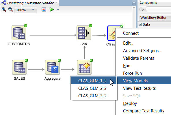
Now, we’ll use the View Models short-cut menu option from the Class Build node to view data about each model individually. In each case, a model window opens that contains four tabs. We’ll examine the Coefficients tab for each model to compare the attributes that are considered significant in predicting the outcome. For all three models, we will look at the Target Value of M (Male).
A. Right-click the Class Build node and select View Models > CLAS_GLM_1_# (the first model, that does not use Feature Selection).
Result: A display window opens with the model name.
B. In the Coefficients tab, perform the following:
The display should look something like this:

Notes:
C. Close the model results display window.
Right-click the Class Build node and select View Models > CLAS_GLM_2_# (the second model, that uses Feature Selection only).
A. In the Coefficients tab, use the same criteria and sorting as with the first model.

Notes: This model indicates only one attributes as primary determining features in the prediction: CUST_MARITAL_STATUS, with the values of "Widowed", "Divorc.", and "Married".
B. View the last model from the Class Build node (View Model > CLAS_GLM_3_#).
Results: The third model generates identical results to the second model. This means that there were no additional features generated out of the source data.
In summary, we can see in this scenario that the feature selection/generation option for GLM provided a high degree of accuracy, without sacrificing the transparency of the model.
Summary
- Add data sources from other schemas
- Use the Aggregate and Join nodes from the Transforms node group
- Copy and modify existing models for comparative purposes
- See the Oracle Data Mining and Oracle Advanced Analytics pages on OTN.
- Refer to additional OBEs in the Oracle Learning Library
- See the Data Mining Concepts manuals:
In this lesson, you learned how to use the Feature Extraction/Generation option with a GLM algorithm classification model.
You also learned how to:
Resources
To learn more about Oracle Data Mining:
Credits
Lead Curriculum Developer: Brian Pottle
Other Contributors: Charlie Berger, Mark Kelly, Margaret Taft, Kathy Talyor
To help navigate this Oracle by Example, note the following:
- Hiding Header Buttons:
- Click the Title to hide the buttons in the header. To show the buttons again, simply click the Title again.
- Topic List Button:
- A list of all the topics. Click one of the topics to navigate to that section.
- Expand/Collapse All Topics:
- To show/hide all the detail for all the sections. By default, all topics are collapsed
- Show/Hide All Images:
- To show/hide all the screenshots. By default, all images are displayed.
- Print:
- To print the content. The content currently displayed or hidden will be printed.
To navigate to a particular section in this tutorial, select the topic from the list.