Using the SQL Query Node in a Workflow
Overview
- Have access to or have installed:
- Oracle Database 12c Enterprise Edition, Release 12.1 with Advanced Analytics Option.
- The Oracle Database sample data, including the unlocked SH schema.
- SQL Developer 4.0
- Set up Oracle Data Miner for use within Oracle SQL Developer 4.0. If you have not already set up Oracle Data Miner, complete the lesson: Setting Up Oracle Data Miner 4.0
- Completed the lesson: Using Oracle Data Miner 4.0
Purpose
This tutorial covers the use of the new SQL Query Node in an Oracle Data Miner 4.0 workflow.
Time to Complete
Approximately 15 mins.
Scenario
This lesson addresses a business problem that can be solved by applying a Classification model. In our scenario, ABC Company wants to predict which customers will have a high life-time value (LTV), based on certain demographic data and other input attributes.
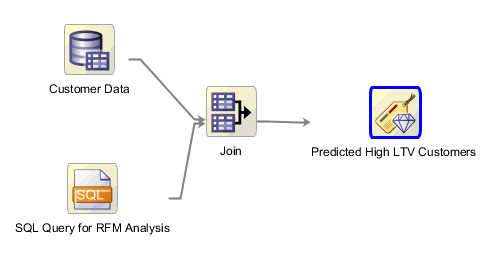
In this lesson, you create a workflow that combines data that is produced from a SQL Query node with data that is defined by a normal data source node. The joined data is then fed to a classification model to generate the predictive results.
The completed workflow looks like this:
Software Requirements
The following is a list of software requirements:
Prerequisites
Before starting this tutorial, you should have:
Create a Data Miner Project
- NOTE: If you have already completed the lesson Using Feature Selection and Generation with GLM, skip this topic go to Build the Data Miner Workflow.
To create a Data Miner Project, perform the following steps:
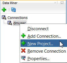
In the Data Miner tab, right-click dmuser and select New Project, as shown here:
In the Create Project window, enter a project name (in this example SH Schema) and then click OK.
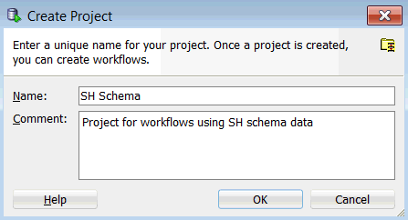
Note: You may optionally enter a comment that describes the intentions for this project. This description can be modified at any time.
Result: The new project appears below the data mining user connection node.
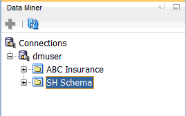
Note: In this image, the project that was created in the "Using Oracle Data Miner 4.0" tutorial is also shown.
Build the Data Miner Workflow
- Joins customer demographic data (from a database table) with aggregated sales data for each customer (geneated by a SQL query).
- Feeds the joined data to a classification build node that is designed to predict which customers are most likely to join the Affinity Card program.
- In the middle of the SQL Developer window, an empty workflow canvas opens with the name that you specified.
- On the upper right-hand side of the interface, the Components tab of the Workflow Editor appears.
- If you have completed the lesson Using Feature Selection and Generation with GLM, then you already have access the SH schema -- skip step 4. and go directly to step 5.
- If you have not completed the lesson Using Feature Selection and Generation with GLM, then continue with step 4.
- Select Customer Data as Source 1, and Query for RFM Analysis as Source 2.
- Select the CUST_ID column from both sources.
- Then, click the Add button to define the Join Columns.
- As seen in the "Using Oracle Data Miner 4.0" lesson, all four classification algorithms are selected by default.
- Next, you will remove two of the model settings and then define the settings for the remaining algorithms.
- Therefore, this classification model will be used to predict which customers are most likely to use an Affinity Card with the company.
- Although not required, it is advised that you define a Case ID to uniquely define each record. This helps with model repeatability and is consistent with good data mining practices.
- When the node runs it builds and tests all of the models that are defined in the node.
- As before, a green gear icon appears on the node borders to indicate a server process is running, and the status is shown at the top of the workflow window.
- Viewing the models individually
- Viewing the test results individually, or comparing the test results together
- The results show that the Decision Tree model produces a higher degree of Predictive Confidence and Average Accuracy. The Overall Accuracy for the SVM model is higher.
- Your Test Results may vary slightly in all cases.
- For the selected model in the upper pane, target value details are provided in the lower pane.
- The correct prediction % for the Target Value of "1" ("Yes" on the Affinity Card) is 87.95% for the SVM model.
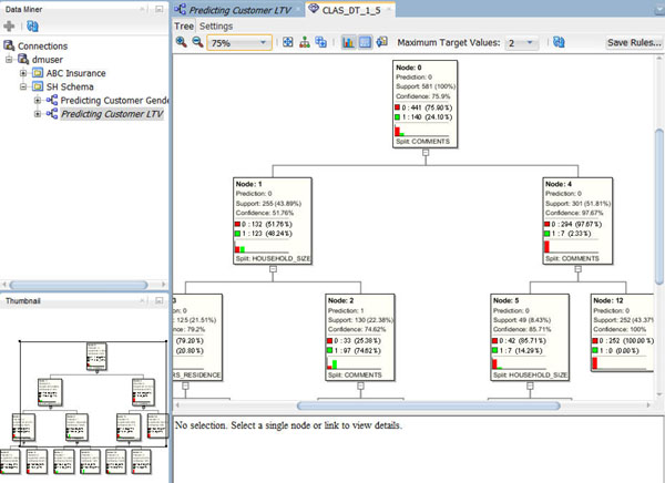
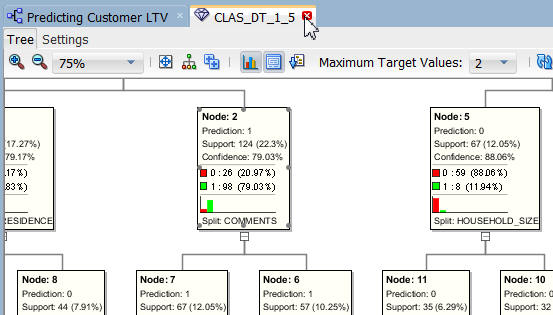
- At each level within the decision tree, an IF/THEN statement that describes a rule is displayed. As each additional level is added to the tree, another condition is added to the IF/THEN statement.
- For each node in the tree, summary information about the particular node is shown in the box.
- In addition, the IF/THEN statement rule appears in the Rule tab, as shown above, when you select a particular node.
- Commonly, a decision tree model would show a much larger set of levels and also nodes within each level in the decision tree. However, the data set used for this lesson is significantly smaller than a normal data mining set, and therefore the decision tree is also small.
- This node indicates that the COMMENTS and HOUSEHOLD_SIZE attributes are the most significant contributors to the prediction.
- In addition, values for each attribute are shown in the Rules tab.
As discussed in the "Using Oracle Data Miner 4.0" tutorial, a Data Miner Workflow is a collection of connected nodes that describe a data mining processes.
Data Mining Scenario
In this topic, you build a workflow that:
Required Task
Before creating the workflow, save RFM-SQL.txt to your local machine. This text document contains a SQL query that you will use for the SQL Query node in the workflow. Make a note of the saved location on your local machine.
To create the workflow for this process, perform the following steps.
Create a Workflow and Add Data Sources
Right-click the SH Schema project and select New Workflow from the menu.
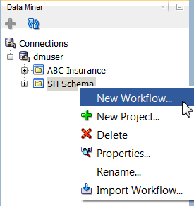
Result: The Create Workflow window appears.
In the Create Workflow window, enter Predicting Customer LTV as the name and click OK.
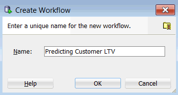
Result:
Next, add a Data Source node to the workflow.
A. In the Components tab, open the Data category.
B. Drag and drop the Data Source node onto the Workflow pane.
Result: A Data Source node appears in the Workflow pane and the Define Data Source wizard opens.
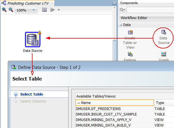
Notes: In the Define Data Source wizard, only tables and views owned by the user are displayed by default. However, for this workflow, you want to use a table in the SH schema.
In Step 1 of the wizard:
A. Click Add Schemas, beneath the Available Tables/Views list, as shown here:
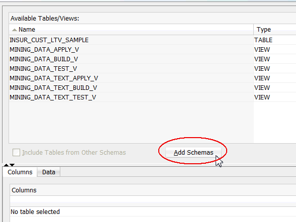
B. In the Edit Schema List window, select SH from the Available Schemas list and move it to the Selected list, as shown below. Then, click OK.
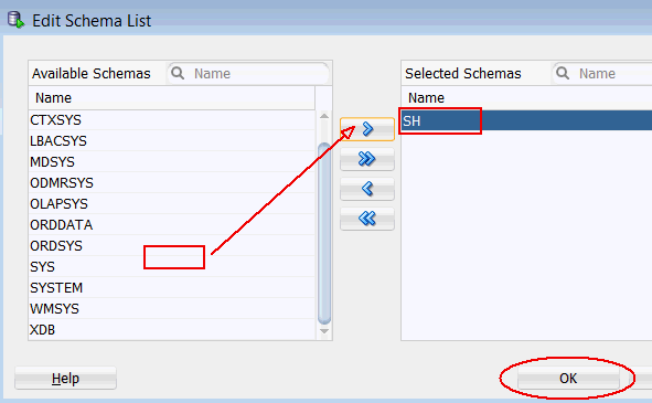
C. Finally, select the Include Tables from Other Schemas option to display the tables and views in the selected schema(s).

Select the SH.SUPPLEMENTARY_DEMOGRAPHICS table and click Finish in the wizard.

Result: A Data Source node for the table is defined in the workflow.
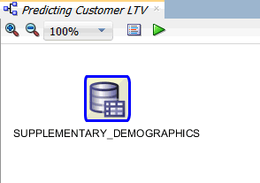
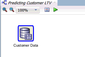
In the workflow, click the node name and change it to Customer Data, like this:
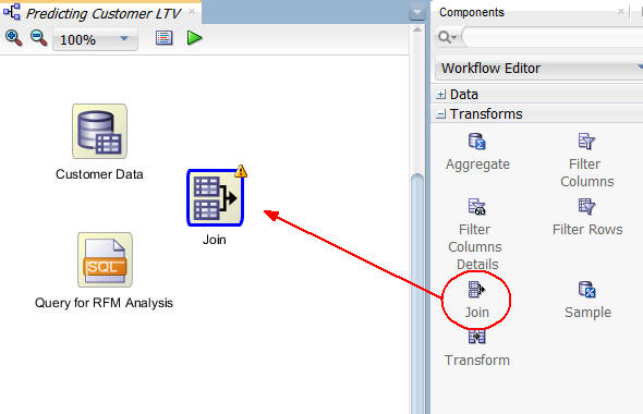
Next, drag and drop a SQL Query node from the Data group to the workflow, just underneath the Customer Data node, like this:

A. In the SQL Developer main menu, select File > Open. Using the Open dialog box, navigate to the location where you saved the RFM-SQL.txt file, select the file, and click Open.
Result: The file is opened in a tabbed window.
B. Select the entire query, as shown below, and copy the selection to the clipboard.
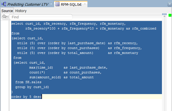
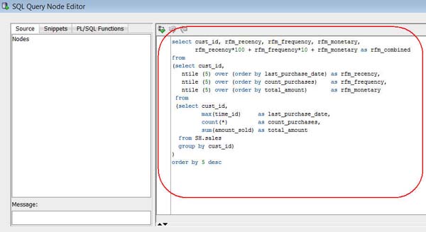
Note: This query uses a nested SELECT statement on the SALES table in the SH schema to aggregate the COUNT_PURCHASES and TOTAL_AMOUNT measures, by the latest purchase date, for each customer.
C. Close the RFM-SQL.txt tabbed window.
D. Double-click the SQL Query node to open the SQL Query Node Editor.
E. Using the Paste short-cut (CTRL+V), paste the code into the SQL Statement pane on the right, like this:
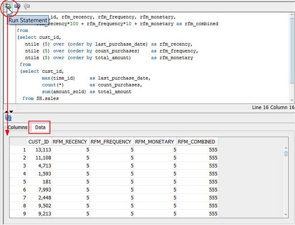
F. Click the Run Statement tool to preview the query results, like this:
G. Click OK to save the SQL Query node.
H. Finally, rename the SQL Query node to Query for RFM Analysis.
Result: The workflow should look like this:

Join the Data
In this topic, you join the customer demographics data to the aggregated sales data defined in the SQL Query node.
Follow these steps:
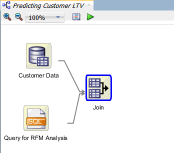
To begin, add a Join node to the workflow and connect the two data nodes to the join node.
A. Open the Transforms group in the Components tab.
B. Drag and drop a Join node onto the workflow, like this:
C. Connect the Customer Data node to the Join node, and then connect the Query for RFM Analysis node to the Join node, like this:

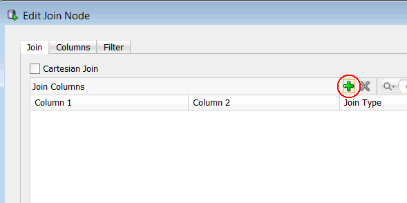
Next, double-click the Join node to display the Edit Join Node window.
A. In the Join tab, click the Add (green "+" icon), like this:
B. In the Edit Join Column window:
The Edit Join Column window should look like this:
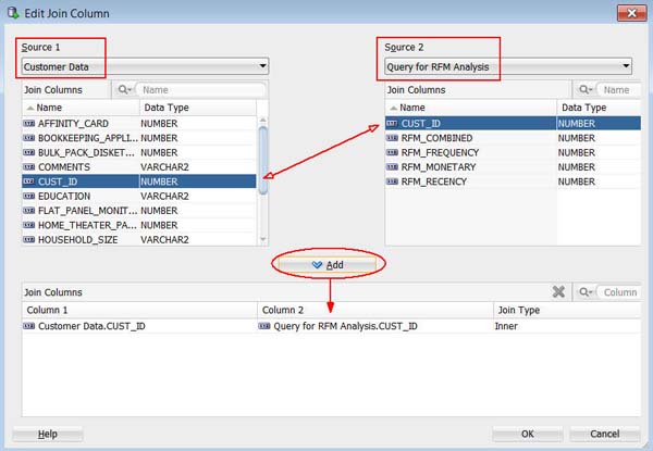
C. Click OK in the Edit Join Column window.
D. Finally, click OK in the Edit Join Node window.
Result: The workflow should now look like this:
Create Classification Models
In this topic, you add a Classification node to the workflow, like you did in the Using Oracle Data Miner 4.0 tutorial. However, in this scenario, you will remove two of the default algorithms from the Class Build node and define only the Decision Tree and SVM models.
Then, in the next topic, you will build the two classification models and compare the results.
Follow these steps:
Add a Classification node to the Workflow, and connect the Join node to it.
A. First, expand the Models category in the Components tab. Then drag and drop the Classification node to the Workflow pane, like this:
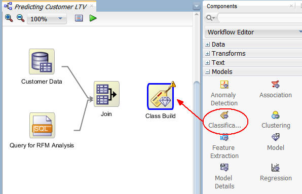
B. Then, connect the Join node to the Class Build node.
Note: When the connection is made, the Edit Classification Build node window appears automatically.
C. Select the Build tab, as shown below.
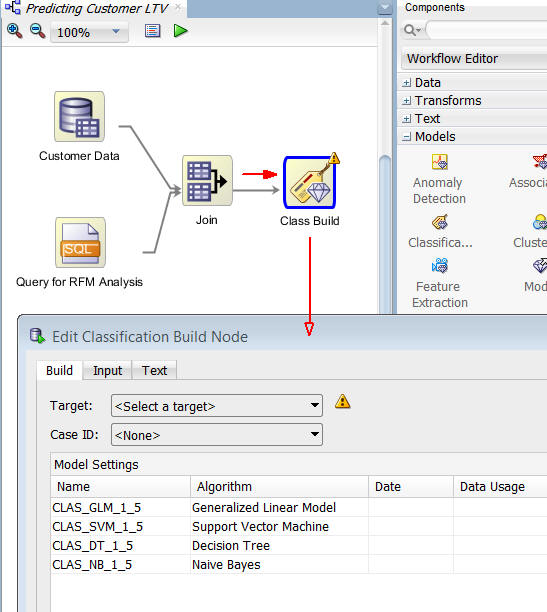
Notes:
Select the CLAS_GLM_#_# and CLAS_NB_#_# model settings. Then click the Remove tool (red "x" icon), as shown below. (Select Yes in the warning message window.)
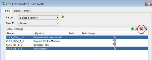
Result: The Support Vector Machine and Decision Tree algorithm model settings remain in the list.
In the Edit Classification Build Node window:
A. Select AFFINITY_CARD as the Target attribute.
B. Select CUST_ID as the Case ID attribute.

Notes:
Next, select the Input tab.
A. De-select the Determine inputs automatically option, as shown here:
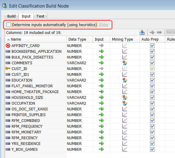
Result: The Input option for all of the attributes except AFFINITY_CARD (the Target) and CUST_ID (the Case ID) may be modified
B. Click the Input icon (green arrow) for the CUST_ID1 and PRINTER_SUPPLIES attributes. In both cases, select the Ignore option (small green arrow followed by a small red "x") in the drop-down list.
Result: These two attributes display the Ignore icon in the Input column, as shown below. This indicates that they will not be used as inputs for the models.

C. Click OK to save these settings and close the Edit Classification Build Node window.
In the workflow, rename the Class Build node to Predicted High LTV Customers, as shown here:

Build and Compare the Models
In this topic, you build the two classification models against the joined source data. Then, you examine the model results.
Right-click the Predicted High LTV Customers node and select Run from the pop-up menu.
Notes:
When the build is complete, all nodes contain a green check mark in the node border.

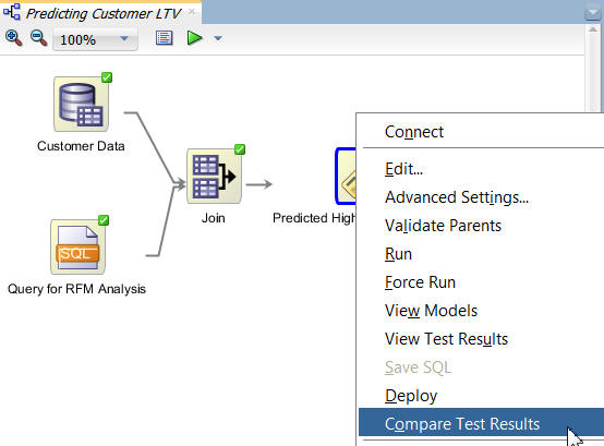
Once the build process is complete, you can compare models by:
Right-click the Class Build node and select Compare Test Results from the menu, like this:
Results: A window opens showing a graphical comparison of the two models in the Performance tab, as shown here:
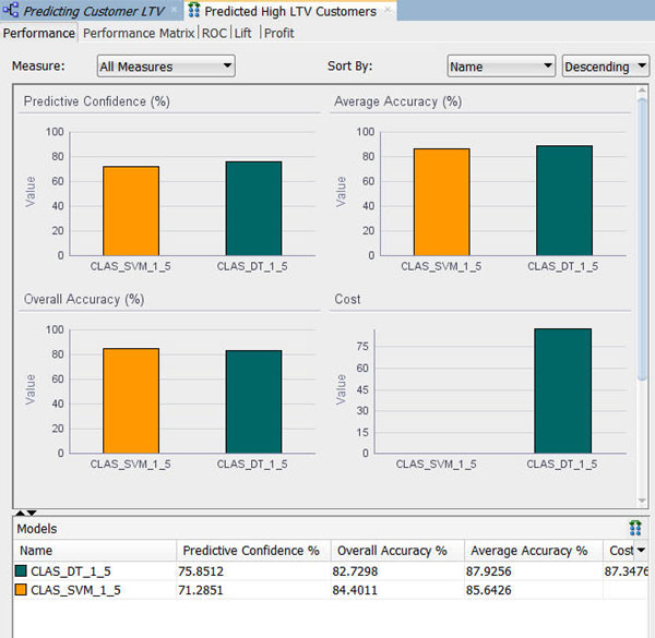
Notes:
Next, select the Performance Matrix tab.
A. Select the SVM model.
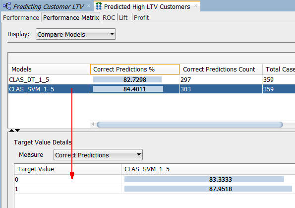
Notes:
B. Select the DT model.
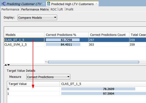
Note: The correct prediction % for the Target Value of "1" ("Yes" on the Affinity Card) is 97.6% for the DT model.
When you are done looking at the Performance Matrix tab, close the Predicted High LTV Customers window.
Next, right-click the Predicted High LTV Customers node and select View Models > CLAS_DT_1_#.
Result: A Decision Tree display window opens with the model name. The display should look something like this:
Navigate to and select Node 2, which is after the second split for a prediction of "1" ("Yes" for the Affinity Card.)
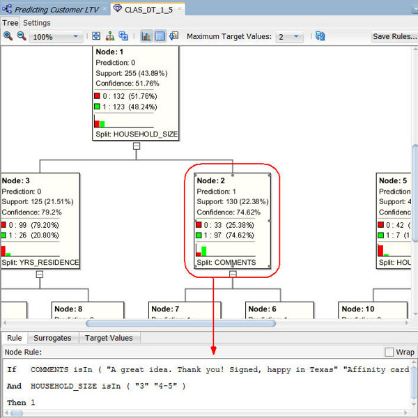
Result:
Conclusion:
Dismiss the Decision Tree display tab as shown here:
Click Save All to save the workflow.
Summary
- Joined customer demographic data (from a database table) with aggregated sales data, as defined in a SQL Query node.
- Fed the joined data to a Classification Model.
- Examined the predictive results.
- See the Oracle Data Mining and Oracle Advanced Analytics pages on OTN.
- Refer to additional OBEs in the Oracle Learning Library
- See the Data Mining Concepts manuals:
In this lesson, you learned how to use the SQL Query node in a workflow. Specifically, you:
Resources
To learn more about Oracle Data Mining:
Credits
Lead Curriculum Developer: Brian Pottle
Other Contributors: Charlie Berger, Mark Kelly, Margaret Taft, Kathy Talyor
To help navigate this Oracle by Example, note the following:
- Hiding Header Buttons:
- Click the Title to hide the buttons in the header. To show the buttons again, simply click the Title again.
- Topic List Button:
- A list of all the topics. Click one of the topics to navigate to that section.
- Expand/Collapse All Topics:
- To show/hide all the detail for all the sections. By default, all topics are collapsed
- Show/Hide All Images:
- To show/hide all the screenshots. By default, all images are displayed.
- Print:
- To print the content. The content currently displayed or hidden will be printed.
To navigate to a particular section in this tutorial, select the topic from the list.