Analyzing Plan Data in Smart View

Before You Begin

This 35-minute tutorial shows you how to analyze plan data using ad hoc grids in Smart View.

Background

Performing Ad Hoc analysis in a form lets you start out focused on the members defined within the form layout. To facilitate your analysis in an adhoc grid, you can control which dimensions members display in the grid and point-of-view (POV).

In this tutorial, learn how to perform ad hoc analysis on plan data:

Apply formatting, data, and member options that emphasize data on your form
Specify dimensions and members displayed in the POV and ad hoc grid by using the keep/remove, pivoting, member selector, and zoom features
Include calculating and non-calculating rows and columns in your ad hoc grid
Preserve Excel formulas in ad hoc grids

What Do You Need?

Have Service Administrator or Ad Hoc Grid Creator role access to Planning for EPM Enterprise Cloud Service Cloud.
Ensure that Microsoft Excel is installed.
Install Oracle Smart View for Office from the Downloads page of Planning or the Oracle Technology Network. Oracle Smart View is an add-in to Microsoft Office products.
Upload and import this snapshot into your Planning instance. The snapshot includes the Quarterly Income Statement form and Planning data required for this tutorial. For more information on uploading and importing migration snapshots, refer to the Administering Migration for Oracle Enterprise Performance Management Cloud documentation.
Ensure that you have your provider configured that connects with a Shared or Private connection to the Planning sample application in your instance.

Connecting to Planning in Smart View

Launch Excel. Ensure that you have a blank worksheet open.
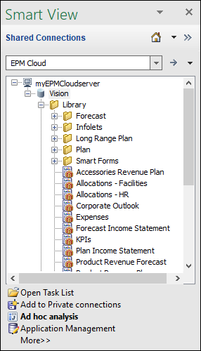
On the Smart View ribbon, click Panel.
Connect to your EPM Cloud instance using Shared Connections, Private Connections, or Recently Used.
Expand the server node.
Expand Vision to display the business process components.

For more information on tasks you can perform with Smart View, see the Working with Oracle Smart View for Office documentation.

Starting Ad Hoc Analysis

In the Smart View panel, under Vision, expand Library, and then Plan.
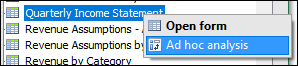
Locate and right-click Quarterly Income Statement, and select Ad hoc analysis.

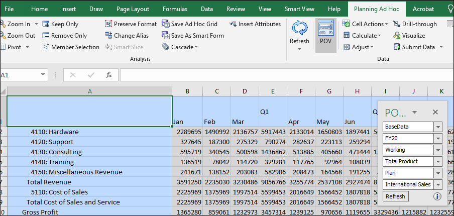
The form is opened in Ad Hoc mode, with the Planning Ad Hoc ribbon selected. The Planning Ad Hoc ribbon provides quick access to ad hoc analysis tasks.

Initially, you see the rows and columns from the form.

There is also a POV (point-of-view) dialog box where you can select members for the POV.

You can dock or hide the POV.
Dock the POV dialog box. Drag and drop the POV dialog box on the Planning Ad Hoc ribbon.
Hide the POV dialog box. Click the (X) Close button in the POV dialog box.
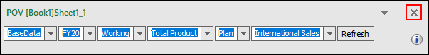
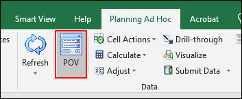
Open the POV dialog box. On the Planning Ad Hoc ribbon, click POV.

Formatting Ad Hoc Grids

You can format your form with the formatting selections made in the Cell Styles and Formatting tabs of the Options dialog box.

Selecting Formatting Options

From the Smart View ribbon, click Options.
From Options, select Formatting in the left pane.
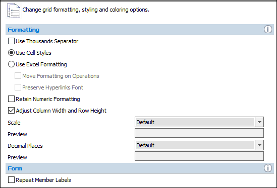
Select a formatting option:
- Use Cell Styles
- Use Excel Formatting
  If you select Excel Formatting, optionally select the following options:
  - Move Formatting on Operations
  - Preserve Hyperlinks Font
  If you select Excel Formatting, Retain Numeric Formatting is disabled.
Select to apply the following options:
- Use Thousands Separator
- Retain Numeric Formatting
- Adjust Column Width and Row Height
Set the Scale to override the setting defined in the form definition. Choose a positive or negative scaling option.
The Preview in the next line displays a sample.
Specify the Decimal Places for the data values.
The Preview in the next line displays a sample.
For Forms, select Repeat Member Labels to allow member names to appear on each row of data.
Click OK.
On the Smart View Ribbon, click Refresh to apply the formatting options to the grid.

Using Excel Formatting

Use formatting to change grid formatting, styling, and coloring options.

If you use Excel formatting, your formatting selections, including conditional formatting, are applied and retained on the grid when you refresh or perform ad hoc operations.

When you use Excel formatting, Smart View does not:

Reformat cells based on your grid operations
Mark cells as dirty when you change data values

Smart View does preserve the formatting on the worksheet between operations.

From the Smart View ribbon, click Options.
From Options, select Formatting in the left pane.
Select Use Excel Formatting.
Optional: Select Move Formatting on Operations.
Optional: Select Preserve Hyperlinks Font.
If you select Excel Formatting, Retain Numeric Formatting is disabled.
Click OK.
On the Smart View Ribbon, click Refresh to apply the formatting options to the grid.

Setting Cell Styles

Use cell styles to indicate certain types of member and data cells.

From the Smart View ribbon, click Options.
From Options, select Formatting in the left pane.
Select Use Cell Styles.
In the left pane, select Cell Styles.
Cell Styles control the display of certain types of member and data cells.
Expand Planning and Common.
Expand Member cells and Data cells.
Because cells may belong to more than one type—a member cell can be both parent and child, for example—you can also set the order of precedence for how cell styles are applied.
Select an object type under Member cells, Data cells, or Common.
Click Properties and select an option: Font, Background, or Border.
- If you selected Font, make your font selections on the Font dialog box and click OK.
- If you selected Background, select a color and click OK.
- If you selected Border, select a color and click OK.
Collapse Planning.
Click OK.
On the Smart View Ribbon, click Refresh to apply the formatting options to the grid.

Cell style options are global options, which apply to the entire current workbook, including any new worksheets added to the current workbook, and to any workbooks and worksheets that are created henceforth. Changes to global option settings become the default for all existing and new Microsoft Office documents.

Setting Data Options

From the Smart View ribbon, click Options.
From Options, select Data Options in the left pane.
Set options for the display of data cells.

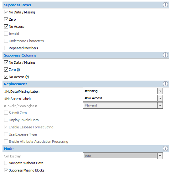
Data options are sheet level options, which are specific to the worksheet for which they are set.
Click OK.
On the Smart View Ribbon, click Refresh to apply the data options to the grid.

Preserving Excel Formulas in Ad Hoc Grids

From the Smart View ribbon, click Options.
From Options, select Member Options in the left pane.
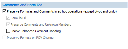
Ensure that Preserve Formulas and Comments in ad hoc operations (except pivot and undo) is selected.
Click OK.

Performing Ad Hoc Analysis

Keeping and Removing Members

You can customize your ad hoc grid by keeping or removing selected members. In this example, you keep the Total Revenue member and remove the first two quarters of the year.

Select the Planning Ad Hoc ribbon.
In the grid, select Total Revenue.
From the Planning Ad Hoc ribbon, click Keep Only.
The grid is updated. Only the current selected member is displayed.
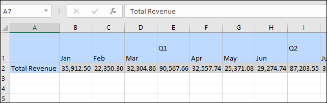
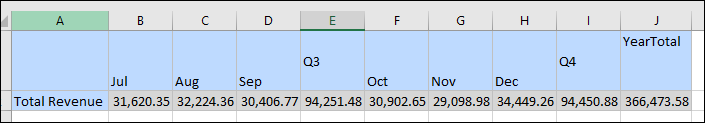
In the grid, select Jan, Feb, Mar, Q1, Apr, May, Jun and Q2.
From the Planning Ad Hoc ribbon, click Remove Only.
The grid is updated. Only the current selected member is displayed.

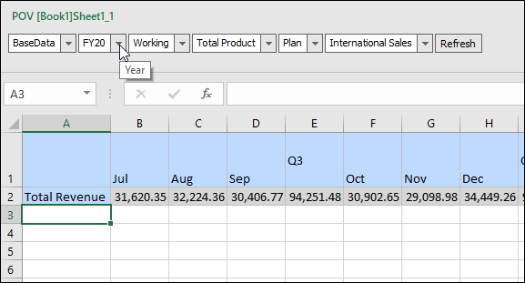
Pivoting Members

You can pivot dimensions to the POV, columns, or rows. The available choices depend on which axis the dimension is located before you pivot it.

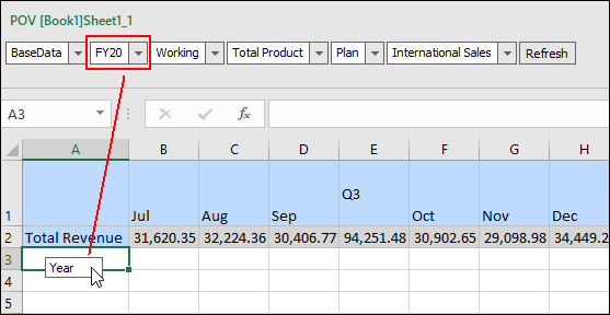
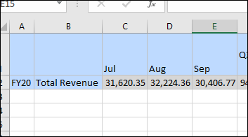
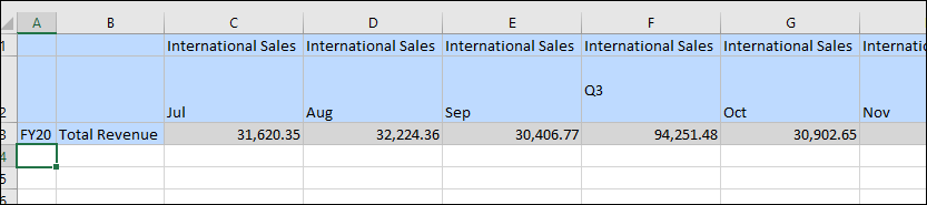
Pivot a dimension from the POV to the rows. From the POV, click and drag the Year dimension (FY20) to the rows.
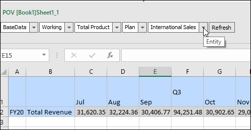
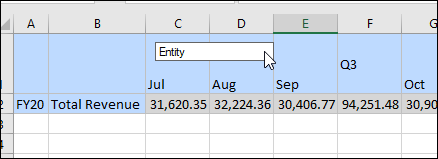
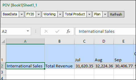
Pivot a dimension from the POV to the columns. From the POV, click and drag the Entity dimension (International Sales) to the columns.
Pivot a dimension that is currently in the rows or columns. In the grid, click International Sales.
From the Planning Ad Hoc ribbon, click Pivot.

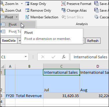
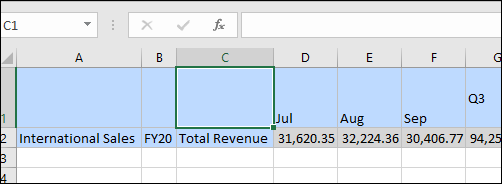
When you select Pivot, if the dimension was in the column, your action moves it to the row. Similarly, if the dimension is in the row, your action moves it to the column.

When you pivot a member, the other members in its dimension are also pivoted.

You cannot pivot the last dimension in a row or column.
In the grid, click the Year dimension (FY20).
Pivot dimensions based on your reporting requirements. For example, if you are analyzing only one year of data, you can pivot the Year dimension back to the POV.
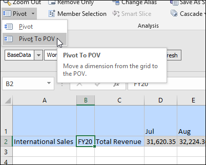
From the Planning Ad Hoc ribbon, click the down-arrow next to Pivot to display options, and select Pivot to POV.

Selecting Members (Member Selector)

You can select members for dimensions in your ad hoc grid by using the Member Selection dialog box.

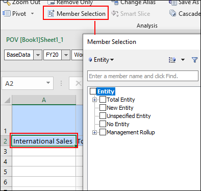
Select members for the Entity dimension. In the grid, select the Entity dimension (International Sales).
From the Planning Ad hoc ribbon, click Member Selection.
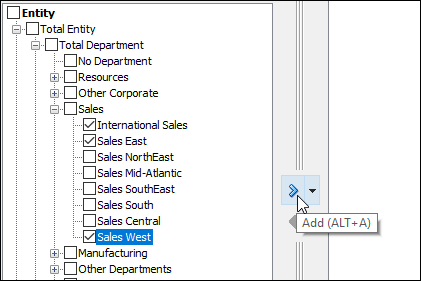
Expand Total Entity, then Total Department, and then Sales.
Select International Sales, Sales East, and Sales West, and then click Add.
Click OK.
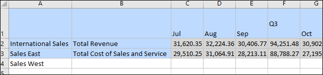
Select members for the Account dimension. In the grid, select the Account dimension cell for Sales East ( B3).
From the Planning Ad hoc ribbon, click Member Selection.
In Member Selection, use the search feature to find members. In the Search field, type Total Cost of Sales and Service and press <Enter>.
Select Total Cost of Sales and Service and click Add.
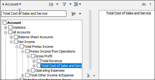
Click OK.
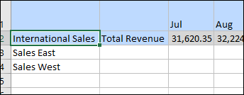
From the Planning Ad Hoc ribbon, click Refresh.
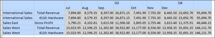
The grid displays data for the selected members.
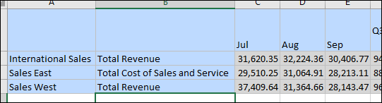
Select an account for Sales West. In the grid, click in the Account dimension cell for Sales West (B4).
Type Total Revenue and press <Enter>.
From the Planning Ad Hoc ribbon, click Refresh.
The grid displays data for the selected members.
Select members for dimensions on the POV. In the POV, click the Product dropdown list and select the ellipsis.
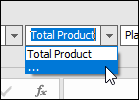
In Member Selection, expand Total Product, then select Computer Equipment.
Click the down arrow next to Add and select Descendants Inclusive.
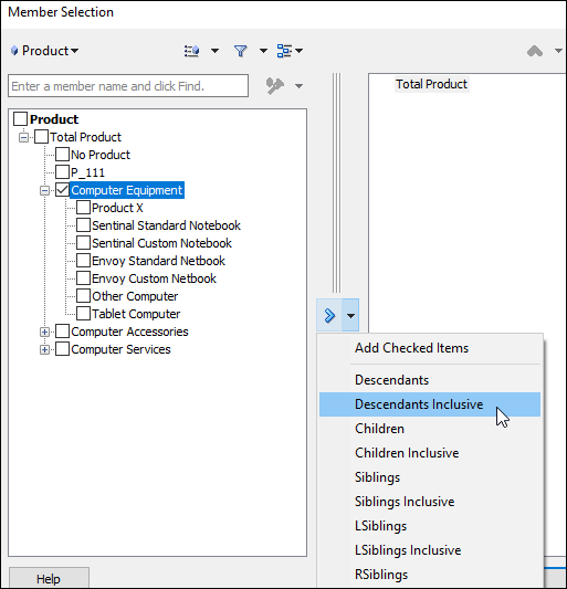
Click OK.
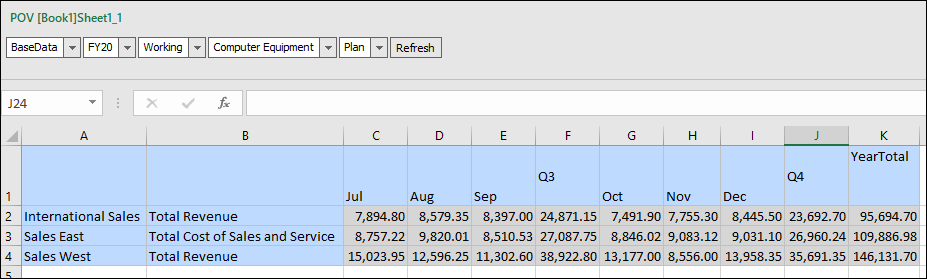
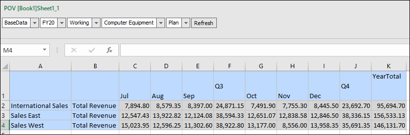
In the POV, click the Product dropdown list to view the updated list of members.
Select Computer Equipment and click Refresh.
The ad hoc grid displays data based on your member selections.

When performing ad hoc analysis, you can use the Insert Attributes option from the Planning Ad Hoc ribbon to insert attribute dimensions or members on the worksheet.

Zooming In and Out Member Levels

You can zoom in and out to display data for different levels in the dimension hierarchy.

In the grid, select the Total Revenue account member for International Sales (B2).
From the Planning Ad hoc ribbon, click the down arrow for Zoom In to display options.
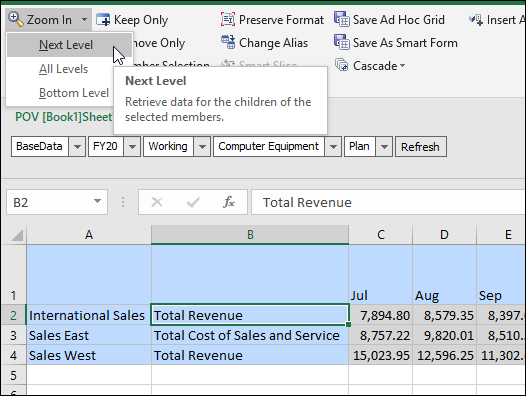
Select Next Level.
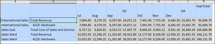
In the grid, select the Total Cost of Sales and Service account member for Sales East (B4).
From the Planning Ad hoc ribbon, click Zoom Out.

Zooming out collapses the view according to the last Zoom In level selection.

Inserting Calculating and Non-Calculating Rows and Columns

You can insert calculating and non-calculating columns and rows within or outside the grid.

Inserted rows and columns, which may contain formulas, text, or Excel comments, are retained when you refresh or zoom in.

See the Preserving Excel Formulas in Ad Hoc Grids section in this tutorial to make sure your associated Excel formulas and comments are saved to the form.

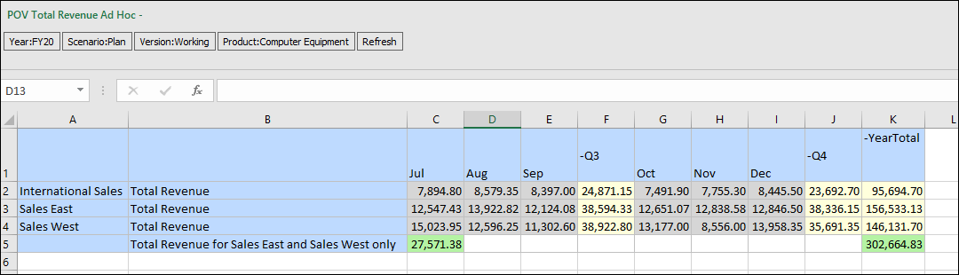
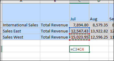
Update the ad hoc grid member selections to display the following example:
In cell C6, enter the following formula: =C3+C4.
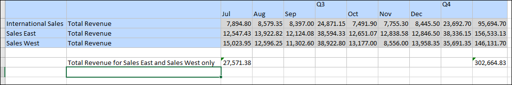
In cell K6, enter the following formula: =K3+K4.
In cell B6, enter the following comment: Total Revenue for Sales East and West only.
From the Planning Ad Hoc ribbon, click Refresh.

Saving Ad hoc Grids as Smart Forms

You can save your ad hoc grid, including the calculations and comments you added, as a Smart Form. Smart Forms support grid labels, along with business calculations in the form os Excel formulas and functions.

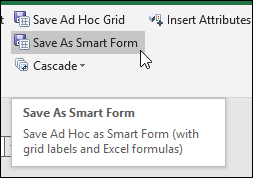
From the Planning Ad Hoc ribbon, click Save As Smart Form.
Enter a Grid Name (form name): Total Revenue Ad Hoc.
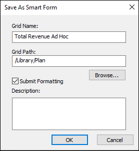
Specify a grid path (form folder): /Library/Plan.
Select Submit Formatting.
This saves any custom Excel formatting changes that have been applied to the grid.
Optional: Enter a description.
Click OK.
The ad hoc grid is saved as a Smart Form.
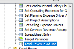
Double-click to open the form.