Before You Begin
Purpose
JSON data can be imported for use with Oracle Data Miner via the new JSON Query node. Once the JSON data is projected to a relational format, it can easily be consumed by Data Miner for graphing, data analysis, text processing, transformation, and modeling.
This tutorial covers the use of the JSON Query Node in an Oracle Data Miner 4.1 workflow in order to mine this Big Data source.
Time to Complete
Approximately 20 mins
Background
JSON is a popular lightweight data structure commonly used by Big Data. For example, web logs generated in the middle tier web servers are likely in JSON format. NoSQL database vendors have chosen JSON as their primary data representation. Moreover, the JSON format is widely used in the RESTful style Web services responses generated by most popular social media websites like Facebook, Twitter, LinkedIn, etc. This JSON data could potentially contain a wealth of information that is valuable for business use.
Oracle database 12.1.0.2 provides ability to store and query JSON data. To take advantage of the database JSON support, Oracle Data Miner 4.1 provides a new JSON Query node that allows users to query JSON data as a relational format.
In additional, the current Data Source and Create Table nodes are enhanced to allow users to specify JSON data in the input data source.
Scenario
In this lesson, you create a workflow that imports JSON data by using the JSON Query node. The JSON Query node enables you to selectively query desirable attributes and project the result in relational format. Once the data is in relational format, you can treat it as a normal relational data source and start analyzing and mining it immediately.
In the workflow, you:
- (A) Identify the JSON data
- (B) Specify the desirable attributes for query purposes
- (C) Examine the JSON data using the JSON Query node
- (D) Build Classification models to provide predictive analysis on the JSON data
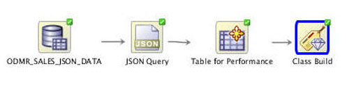
The completed workflow looks like this:
Context
Before starting this tutorial, you should have set up Oracle Data Miner for use within Oracle SQL Developer 4.1, by completing the Setting Up Oracle Data Miner 4.1 tutorial.
In addition, if you are new to Oracle Data Miner, we strongly suggested that you complete the Using Oracle Data Miner 4.1 tutorial.
What Do You Need?
Have access to or have Installed the following:
- Oracle Database: Minimum: Oracle Database 12c Enterprise Edition, Release 1.0.2 (12.1.0.2.0) with the Advanced Analytics Option.
- The Oracle Database sample data, including the SH schema.
- SQL Developer 4.1
Create a Data Miner Project
In the Using Oracle Data Miner 4.1 tutorial you learned how to create Data Miner Project and Workflow.
To create a Data Miner Project for this workflow, perform the following steps:
-
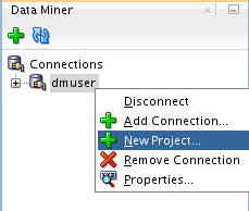
First, select the Data Miner tab. The dmuser connection that you created previously appears.
-
Right-click dmuser and select New Project from the menu.
-
In the Create Project window, enter Big Data Analysis as the project name and then click OK.
Result: The new project appears below the connection node.
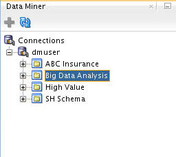
Note: The other projects were created in previously completed turorials.
Build the Data Miner Workflow
As discussed in the Oracle Data Miner 4.1 tutorial, a Data Miner Workflow is a collection of connected nodes that describe a data mining processes.
To create the workflow for this process, perform the following steps.
Create a Workflow and Add the Data Source
-
Right-click the Big Data Analysis project and select New Workflow from the menu.
-
In the Create Workflow window, enter JSON Attribute Analysis as the name and click OK.
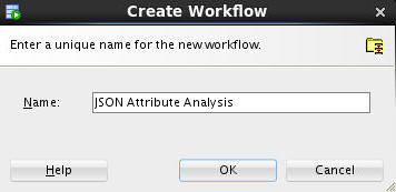
Description of this image Result: Just like in the Using Oracle Data Miner 4.1 tutorial, an empty workflow tabbed window opens with the Workflow name that you specified.
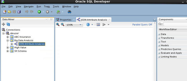
Note: In this example, the other projects were previous created by completing other tutorials in this suite.
-
Next, add a Data Source node for the JSON data.
A. In the Components tab, open the Data category.
B. Drag and drop the Data Source node onto the Workflow pane. Result: The Define Data Source wizard opens automatically.
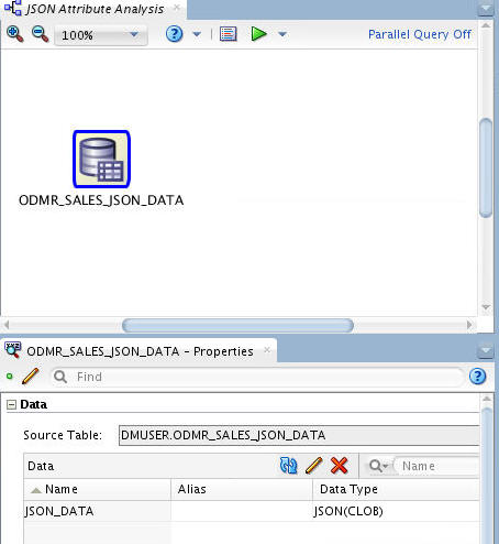
C. In the Available Tables/View list, scroll down and select the ODMR_SALES_JSON_DATA table as shown here:
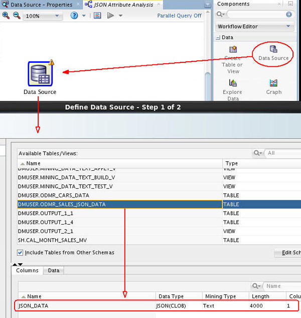
Notes:
- Notice that there is only one column (JSON_DATA) in this table, of JSON(CLOB) data type. The JSON prefix indicates that the data stored is in JSON format, and that CLOB is the original data type.
- This table is installed as part of the demo data that is provided by the Oracle Data Miner.
-
Next, right-click the data source node and select Run from the menu.
Result: When a JSON data source node is run, the execution process parses the JSON documents to produce a relational schema that represents the JSON document structure.
Note: The Data Source node recognizes that the CLOB is json is due to an IS_JSON constraint that has been added to the column definition of the table
-
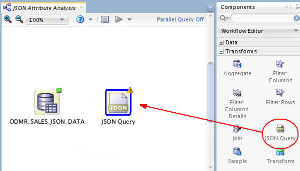
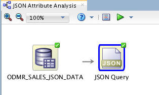
Now, drag and drop a JSON Query node from the Transforms group to the workflow.
-
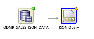
Connect the data source node to the JSON Query node,like this:
-
Double-click the JSON Query node to open the JSON Query Node Editor window.
A. Then, select JSON_DATA as the Column:
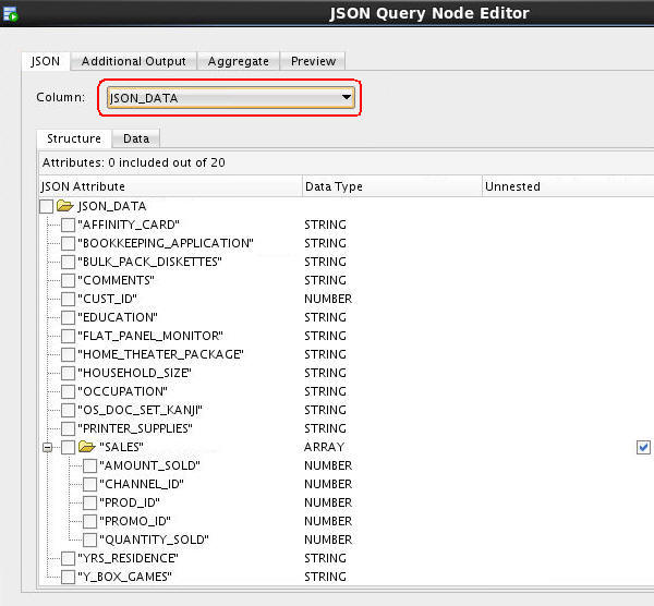
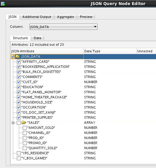
Results: The available JSON attributes are listed in the Structure tab.
B. Select all of the JSON attributes down to, but not including SALES. Note: You will define aggregations for two of the SALES nexted attributes (QUANTITY_SOLD and AMOUNT_SOLD).
-
Next, select the Aggregate tab. Here, you will define aggregations for QUANTITY_SOLD and AMOUNT_SOLD attributes (within the SALES array).
A. First, click the Edit Attribute tool (pencil icon) in the Group By Attributes region.
B. In the Edit Group By window, select CUST_ID as the Group-By attribute, as shown below. (Notice the Group-By attribute can consists of multiple attributes.)
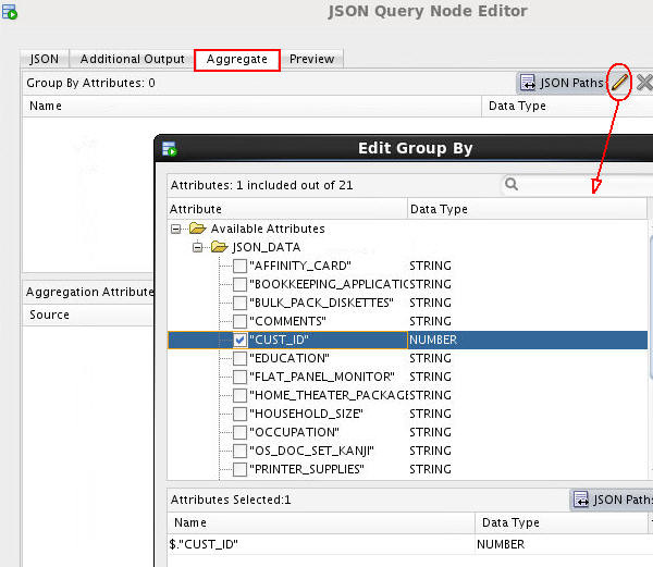
C. Click OK to return to the Aggregate tab.
D. Now, click the Add Attribute tool (green "+" icon) in the Aggregation Attributes region.
E. In the Add Aggregations Dialog window, scroll down and select both the AMOUNT_SOLD and QUANTITY_SOLD attributes. Then click the Formula tool and select SUM from the list as the aggregation function.
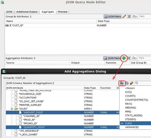
F. Next, click the Sub-Group By Element tool (next to the Formula tool) and select PROD_ID from the list. This selection specifies calculation of quantity sold and amount sold per product per customer.
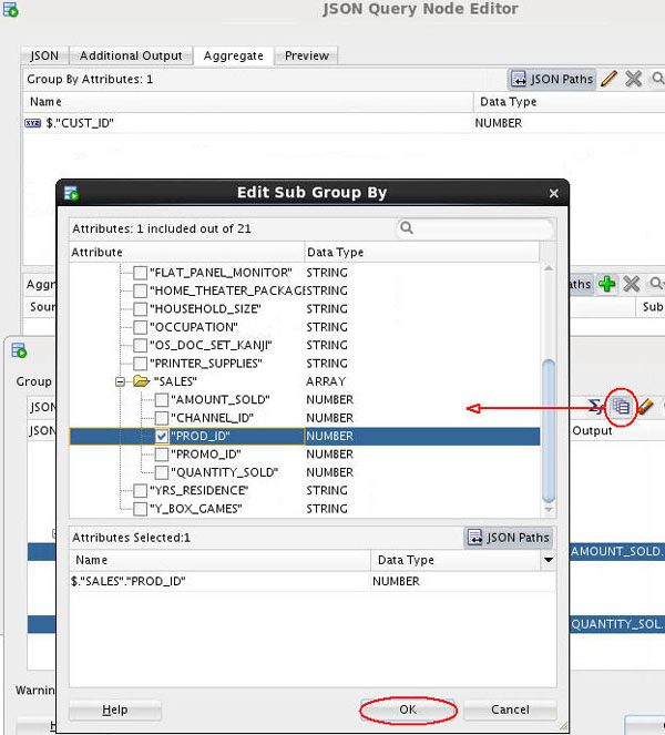
Note: Specifying a Sub-Group By column creates a nested table, and the nested table contains columns with data type DM_NESTED_NUMERICALS.
G. Click OK to return to the Add Aggregates Dialog.
F. Click OK again to return to the JSON Query Node Editor, which should look like this:
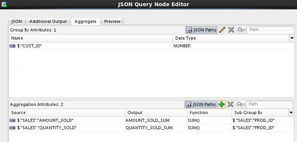
Notes: The Preview tab displays the generated relational output.
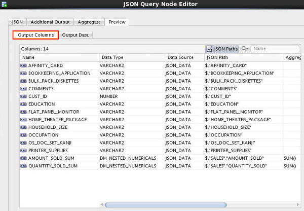
The Output Columns tab shows all output columns and their corresponding source JSON attributes, as shown here. (The output columns can be renamed by using the in-place edit control.)
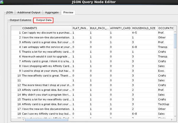
The Output Data tab shows the actual data in the generated relational output.
-
Click OK to close the JSON Query Node Editor.
-
Finally, right-click the JSON Query node and select Run from the menu.
When the process is complete, the workflow should look like this:
Notes: The generated relational output is single-record case format; each row represents a case. If we had not defined the aggregations for the JSON array attributes, the relational output would have been in multiple-record case format, which is not suitable for building mining models except for an Association model.
In this topic, you will create a workflow and add the JSON data source.
D. Click Finish to at the data source node to the workflow.
Create Classification Models
In this topic, first you add a table node to the workflow to persist the JSON Query results. Then you define classification models for the JSON data by using a Classification node.
-
Add a Create Table node to the workflow.
A. Drag and drop a Create Table node to the workflow, like this:

B. Connect the JSON Query node to the OUTPUT node.
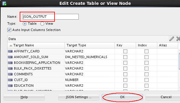
C. Double-click OUTPUT node, and change the table name to JSON_OUTPUT. Then click OK.
D. Finally, rename the OUTPUT node to Table for Performance.
Result: The workflow should look like this:
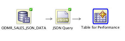
Note: This practice enhances performance when building models against the JSON data.
-
Now, add a Classification node to the workflow.
A. First, expand the Models category in the Components tab. Then drag and drop the Classification node to the Workflow pane, like this:
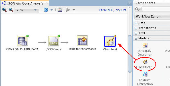
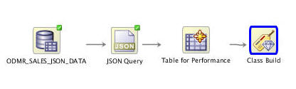
B. Next, connect the Table for Performance node to the Class Build node. (The Edit Classification Build Node window automatically appears.)
-
In the Build tab of the Edit Classification Build Node window:
A. Select AFFINITY_CARD as the Target attribute, and CUST_ID as the Case ID attribute.
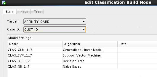
B. Click OK to save these settings and close the Edit Classification Build Node window.
Result: The workflow should now look something like this:
Build and Compare the Models
In this topic, you build the classification models against the structured JSON data. Then, you examine the model results.
-
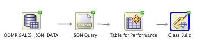
Right-click the Class Build node and select Run from the menu.
Results: When the build is complete, all nodes contain a green check mark in the node border.
-
Right-click the Class Build node and select Compare Test Results from the menu.
Results: A window opens showing a graphical comparison of the models in the Performance tab, as shown here:
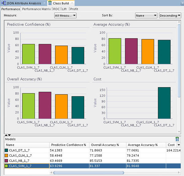
Notes: The results show that the Naive Bayes and SVM models produce a higher degree of Predictive Confidence, Average Accuracy, and Overall Accuracy than the other two model types. (Your Test Results may vary slightly in all cases.)
-
Select the Performance Matrix tab and perform the following:
A. Select the SVM model.
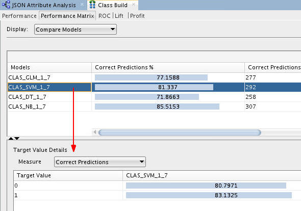
Notes: For the selected model in the upper pane, target value details are provided in the lower pane. The correct prediction % for the Target Value of "1" ("Yes" on the Affinity Card) is 83.13% for the SVM model.
B. Select the NB model.
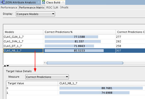
Notes: The correct prediction % for the Target Value of "1" ("Yes" on the Affinity Card) is 74.69% for the NB model.
-
When you are done looking at the Performance Matrix tab, close the Class Build window.
-
Next, right-click the Class Build node and select View Models > CLAS_SVM_1_#
Result: A window opens with statistical analysis of the attributes that are most important in predicting the target (Affinity Card) by using the SVM model. In the Coefficients tab, de-select the Sort by absolute value option, and then sort in descending order using the Coefficient column, as shown here.
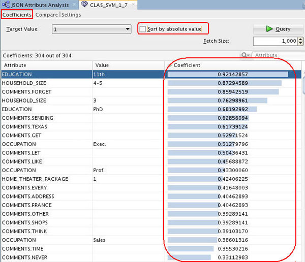
Conclusion: The SVM model indicates that the EDUCATION and HOUSEHOLD_SIZE attributes are the most significant contributors to the prediction. Notice that four of the top five predictive attributes are these two.
-
Dismiss the Decision Tree display tab and close the workflow when you are done viewing the Decision Tree display.