Before You Begin
Purpose
This tutorial covers the use of Predictive Queries against mining data by Oracle Data Miner 4.1.
Time to Complete
Approximately 30 mins
Background
As you learned in the lesson Using Oracle Data Miner 4.1, data mining is the process of extracting useful information from masses of data by extracting patterns and trends from the data.
Data mining can be used to solve many kinds of predictive analysis problems, including the following:
- Predicting outcomes or values (Classification or Regression models)
- Finding natural segments or clusters in a population (Clustering models)
- Finding fraudulent or rare events (Anomaly Detection models)
- Creating new attributes (features) for a target variable by combining original attributes (Feature Extraction models)
Oracle Data Miner provides predictive query capabilities for these specific model types. The predictive query options enable dynamic scoring of these model by generating a transient model that is not persisted.
In this lesson, you will learn how to use each type of predictive query.
Context
Before starting this tutorial, you should have set up Oracle Data Miner for use within Oracle SQL Developer 4.1, by completing the Setting Up Oracle Data Miner 4.1 tutorial.
In addition, if you are new to Oracle Data Miner, we strongly suggested that you complete the Using Oracle Data Miner 4.1 tutorial.
What Do You Need?
Have access to or have Installed the following:
- Oracle Database: Minimum: Oracle Database 12c Enterprise Edition, Release 1.0.2 (12.1.0.2.0) with the Advanced Analytics Option.
- The Oracle Database sample data, including the SH schema.
- SQL Developer 4.1
Creating Predictive Queries
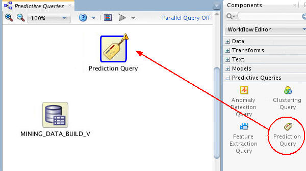
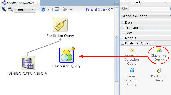
Before getting started, let’s preview the Predictive Queries node group in the Components pane. As shown below, the Models and Predictive Queries node groups are opened.
There are four options in the Predictive Queries node group:
- Anomaly Detection Query
- Clustering Query
- Feature Extraction Query
- Prediction Query
As shown in the image, each Predictive Query option enables dynamic scoring of an associated model type or types.
Open the first subtopic to begin.
Create a Workflow and Add a Data Source
As you learned previously, a Data Miner Workflow is a collection of connected nodes that describe a data mining process. Here, you add a new workflow to an existing project that you created in the "Using Oracle Data Miner 4.1" tutorial. Then, you add a data source to the workflow.
-
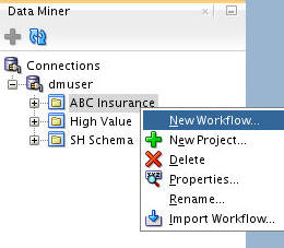
Right-click your project (ABC Insurance) and select New Workflow from the menu. Note: if you have not created this project, follow the simple instructions in the first topic of the "Using Oracle Data Miner 4.1" tutorial.
-
In the Create Workflow window, enter Predictive Queries as the name and click OK.
Result: In the middle of the SQL Developer window, an empty workflow canvas opens with the workflow name that you specified, and the Components tab of the Workflow Editor appears, as you have seen before.
-
As always, start with one or more data sources.
A. In the Components tab, drill on the Data category, drag and drop a Data Source node on the workflow, and select MINING_DATA_BUILD_V from the Available Tables/Views list in the wizard, as shown here:
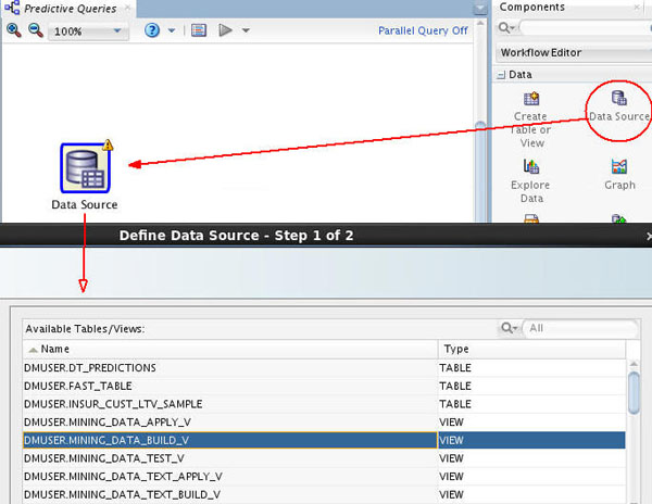
B. Then, click Finish to complete the data source node definition and close the wizard.
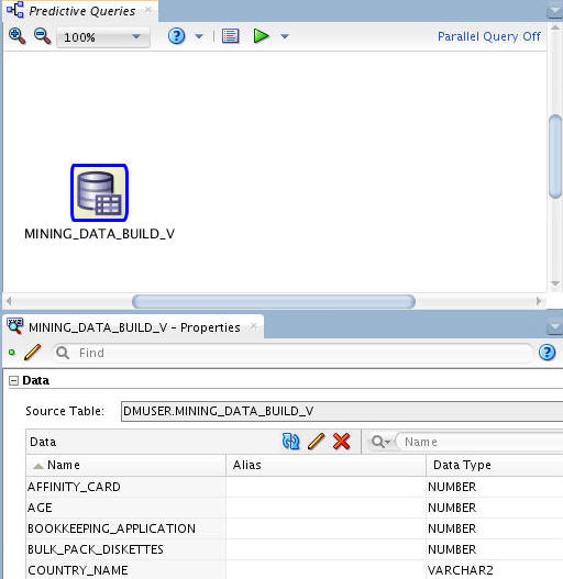
Result: As shown below, the data source node name is updated with the selected table name. Also, in our example we have placed the the Properties tab below the workflow pane.
Note: You will use this same data source for all four predictive query options. Therefore, you will not need to create an additional workflow, nor add additional data sources, to complete this tutorial.
Create and Execute a Prediction Query
When creating a Classification or a Regression model, you must define a target attribute for the prediction. Predictive results are generated by the model and placed in the target attribute for each case in the model scoring process.
When defining a Prediction Query node, you specify one or more prediction targets, which serve as the equivalent of a target attribute in a Classification or Regression model. Then, when the Prediction Query option is run, the Data Mining engine performs dynamic scoring for the prediction target(s) by generating a transient model that is not persisted.
In this topic, you define a Prediction Query node to predict those customers who are most likely to select an Affinity card with the company. Then, you run the node and view the results.
-
Add a Prediction Query node to the workflow.
A. First, collapse the Data category, and open the Predictive Queries category in the Components tab.
B. Then, drag and drop the Prediction Query node from the Components tab to the Workflow pane, like this:
-
Connect the data source node to the Prediction Query node like this:
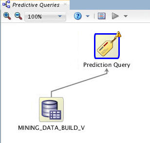
Note: By connecting these nodes, you enable the definition of the Prediction Query options based on the source data.
A Prediction Query node is defined by specifying the following:
- First, define the Case ID attribute.
- Second, add one or more target columns.
- Optionally, select one or more partition columns.
- Optionally, add or remove prediction output columns.
- Optionally specify advanced settings.
-
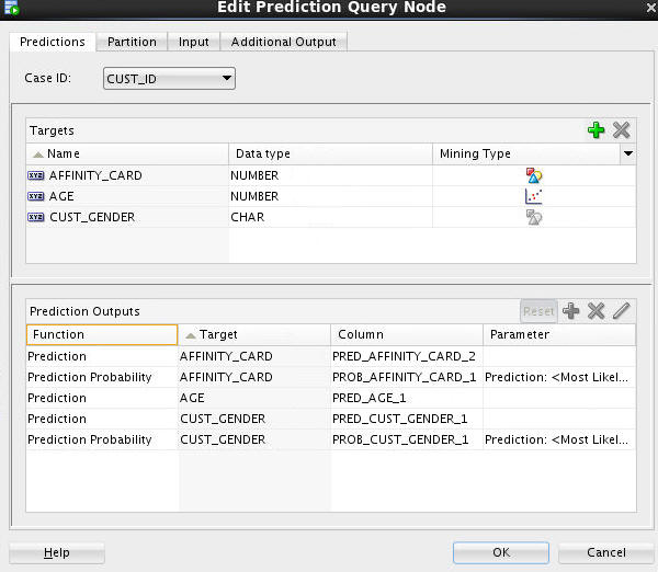
Double-click the Prediction Query node to open the Edit Prediction Query Node window. Then, perform the following:
A. On the Predictions tab, select CUST_ID as the Case ID attribute.
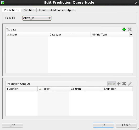
B. Next, add three prediction target attributes as specified here:
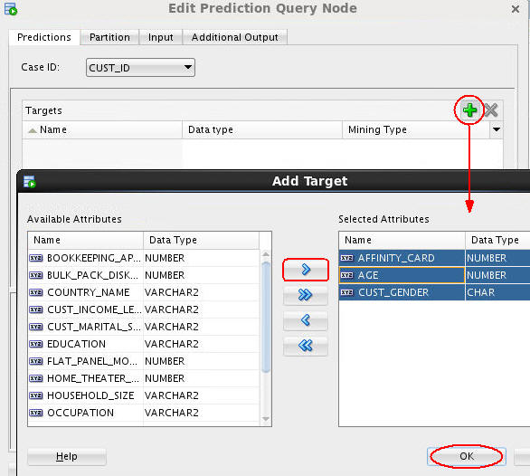
- Click the Add Prediction Target tool (green “+” icon). The Add Target dialog box appears.
- In the Available list, select the AFFINITY_CARD, AGE, and CUST_GENDER attributes to serve as a prediction targets.
- Move the chosen attributes to the Selected list.
- Then, click OK.
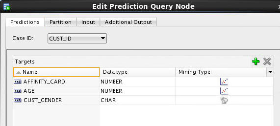
Result: The Targets region of the Predictions tab should look like this:
Notes:
- As stated previously, the Prediction Query feature supports dynamic scoring for both Regression and Classification modeling. As shown in the Targets list on the Prediction tab, each attribute has an associated data type and mining type.
- The mining type defines how the attribute is treated in the analytic query:
- For Regression query analysis, the mining type should be set to Numerical

- For Classification query analysis, the mining type should be set to Categorical

- For Regression query analysis, the mining type should be set to Numerical
In the example, AFFINITY_CARD and AGE are both Numerical, and CUST_GENDER is Categorical, as a result of the associated data types. However, we want to perform classification analysis on AFFINITY_CARD, because we are attempting to predict a Yes (1) or No (0), rather than a number. You can change the mining type of any attribute with a NUMBER data type as desired.
-
Now, change the mining type for the AFFINITY_CARD attribute from Numerical to Categorical.
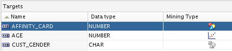
A. For the AFFINITY_CARD target, click the Mining Type icon and select Categorical from the drop-down list, as shown here:

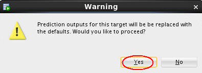
B. The following Warning window opens when you change the Mining Type value. Click Yes.
Result: The prediction targets are now defined correctly for the Prediction Query.
-
Next, click the Partition tab.
Notes: If you select a Partition column, the predictive query builds a model for each unique partition. You may select one or more partition columns. Ensure that the level of partitioning does not get so small that there is insufficient data to build a good model.
Define the following partition column:
A. Click the Add Partitioning Columns tool (green “+” icon). The Add Partition Column dialog box appears.
B. Select the EDUCATION attribute in the Available list and move it to the Selected list.
C. Finally, click OK.
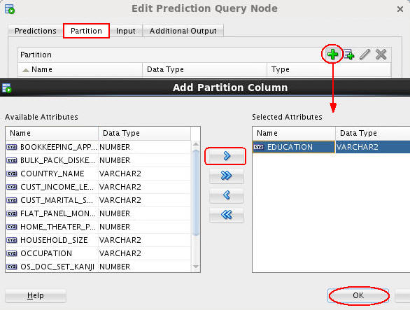
Note: This definition instructs the Data Mining server to build a unique model for each distinct EDUCATION value. Because the model uses data only from that partition, it can potentially predict cases more accurately than if no partition were selected.
-
Select the Input tab. All of the input columns are listed.
By default, inputs are automatically determined using heuristics. If you want to remove or modify the mining type of any input column, you must deselect this option.
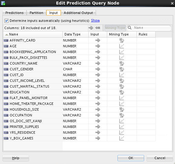
Note: The Additional Output tab enables you to add (or remove) columns to the predictive output that is automatically generated by the node.
-
Once again, select the Predictions tab and examine the Prediction Outputs region at the bottom of the tabbed pane.
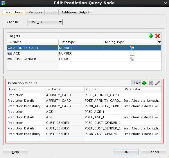
Notes: By default, three prediction output columns are generated for a target attribute with a Categorical mining type (AFFINITY_CARD and CUST_GENDER), and two output colums generated for a target with a Numerical mining type (AGE). You can add or remove prediction output columns.
-
For this analytic query, remove the Prediction Details outputs for all three targets by performing the following:
A. Select the three Prediction Details functions in the Prediction Outputs pane.
B. Click the Remove Prediction Output Function tool (red “x” icon).
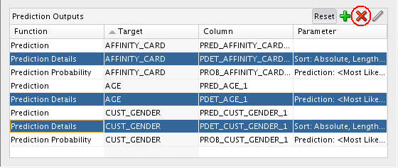
Result:
Note: The column names for your Prediction Outputs are automatically generated, and may be different from those shown in this example.
-
Click OK to close the Edit Prediction Query Node window.
-
To execute the prediction query and view the results, right-click the Prediction Query node and select either Run or View Data from the menu. In this example, we select the View Data option.
Notes: Given that models may take a while to be formulated, running a query may take a while. However, the View Data option generates a smaller sample output of the query.
Result: A Prediction Query tabbed window opens with a small sample of query output, including all of the Additional Output columns and the Prediction Output columns.
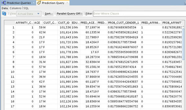
Notes:
- Although you are only viewing the first few rows of the query result, the analytic query processes all the data in the query.
- Your prediction column names may be slightly different.
- In the example, output columns have been resized to provide a more complete view of the results. You can scroll horizontally and vertically to view more of the prediction query data.
-
Click the Sort button and specify the following criteria:
A. Prediction Affinity Card, in Descending order (1 is YES, 0 is NO), and then,
B. Probability Affinity Card, in Descending order (the higher the number, the greater probability of the prediction).
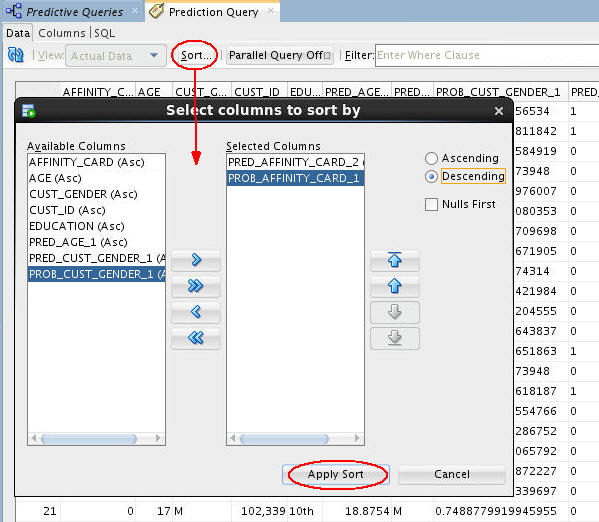
C. Click Apply Sort to view the results.
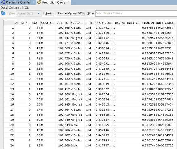
Notes:
- The sorted results show customers sorted by with the highest probability of choosing an Affinity Card.
- This information could be used for a targeted affinity card promotion -- to those customers in this list that don't already have an affinity card.
-
Close the Prediction Query tabbed window and Save the workflow by clicking the Save All icon in main toolbar.
Create and Execute a Clustering Query
Clustering models define segments, or “clusters,” of a population and then decide the likely cluster membership of each new case (although it is possible for an item to be in more than one cluster).
These models use descriptive data mining techniques, but they can be applied to classify cases according to their cluster assignments
When defining a Clustering Query node, you specify similar attributes to a Clustering model, but when the Clustering Query option is run, the Data Mining engine performs dynamic scoring of the clustering query without having to pre-define a model.
In this topic, you define a Clustering Query node to predict homogeneous clusters of customers partitioned on their Country of residence level. Then, you run the node and view the results.
-
Add a Clustering Query node to the workflow, as shown here:
-
Connect the data source node to the Clustering Query node like this:
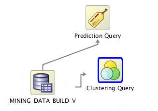
Note: By connecting these nodes, you enable the definition of the Clustering Query options based on the source data.
A Clustering Query node is defined by specifying the following:
- First, define the Case ID attribute.
- Second, specify the number of clusters.
- Optionally, select one or more partition columns.
- Optionally, add or remove prediction output columns.
-
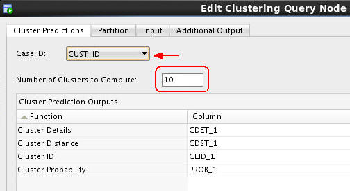
Double-click the Clustering Query node to open the Edit Clustering Query Node window. Then, perform the following on the Predictions tab:
A. Select CUST_ID as the Case ID attribute.
B. Accept the default value of 10 for number of clusters to compute.
-
Next, select the COUNTRY_NAME attribute as the Partition column, as shown here:
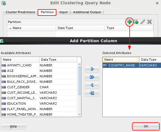
Note: This definition instructs the Data Mining server to build a unique virtual model for each distinct COUNTRY_NAME value.
-
Click OK to close the Edit Clustering Query Node window.
-
Right-click the Clustering Query node and select View Data from the menu.
Result: A tabbed window displays the data, including: Output Columns (CUST_ID, COUNTRY_NAME) and Cluster Prediction Outputs (CLID_1, PROB_1, CDET_1, CDST_1)
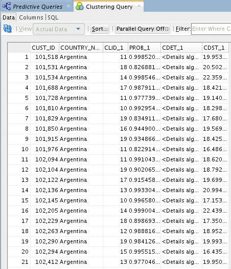
Notes: Your prediction column names may be slightly different. In the example, output columns have been resized.
-
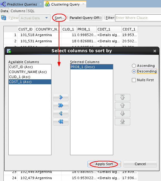
Next, sort and filter the output as follows:
A. Click the Sort button, sort by Probability in Descending order, and then click Apply Sort.
B. Next, apply the following Where clause in the Filter box: CLID_1 = 8
Note: Make sure to use the correct column name from your example in the Filter box.
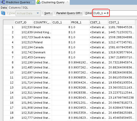
Result: The filter selects only those records that are predicted to be in the eighth cluster.
-
Close the Clustering Query tabbed window and Save the workflow by clicking the Save All icon in main toolbar.
Create and Execute an Anomaly Detection Query
Anomaly Detection models use one-class classification. In this approach, the model trains on data that is homogeneous. Then, the model determines whether a new case is similar to the cases observed, or is somehow “abnormal” or “suspicious.”
When defining an Anomaly Detection Query node, you specify similar attributes to an Anomaly Detection model, but when the query option is run, the Data Mining engine performs dynamic scoring of the anomaly detection query without having to pre-define a model.
In this topic, you define an Anomaly Detection Query node to predict potentially anomalous cases, and view the supporting prediction details.
-
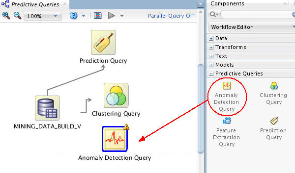
Add an Anomaly Detection Query node to the workflow, as shown here:
-
Connect the data source node to the Anomaly Detection Query node like this:
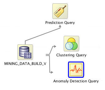
Note: By connecting these nodes, you enable the definition of the Anomaly Detection Query options based on the source data.
An Anomaly Detection Query node is defined by specifying the following:
- First, define the Case ID attribute.
- Second, optionally, select one or more partition columns.
- Third, optionally, add or remove prediction output columns.
-
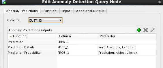
Double-click the Anomaly Detection Query node to open the Edit Anomaly Detection Node window. Then, on the Anomaly Predictions tab, select CUST_ID as the Case ID attribute.
-
Next, select the COUNTRY_NAME attribute as the Partition column, as shown here:
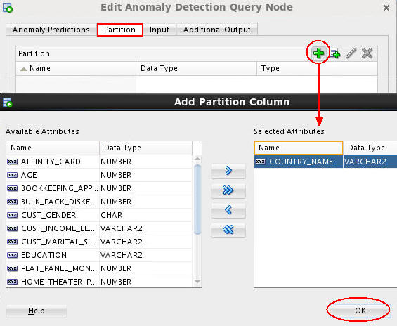
Note: This definition instructs the Data Mining server to build a unique model for each distinct COUNTRY_NAME value.
-
Click OK to close the Edit Clustering Query Node window.
-
Right-click the Clustering Query node and select View Data from the menu.
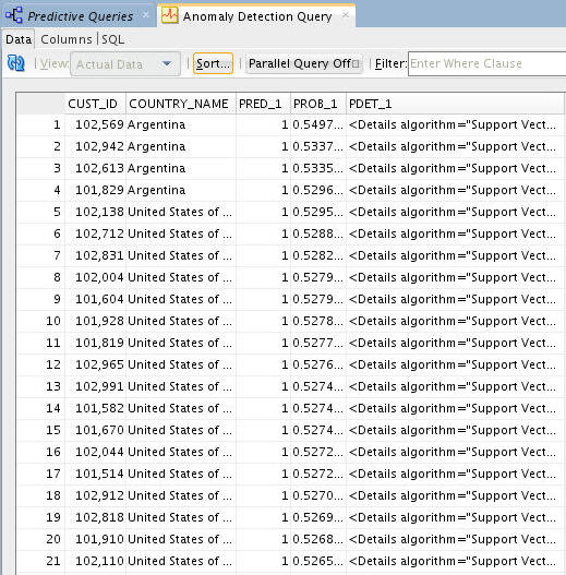
Result: A tabbed window displays the data, including: Output Columns (CUST_ID, COUNTRY_NAME) and Anomaly Prediction Outputs (PRED_1, PROB_1, PDET_1).
-
Sort the query results using the following criteria:
A. Prediction, in descending order.
B. Probability, in descending order.
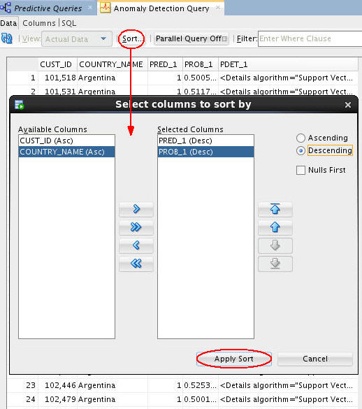
C. Then click Apply Sort for view the sorted data, which is shown here:
-
The Anomaly Prediction Query options enable viewing of expanded prediction details. Perform the following:
A. First, click the PDET_# column for the case you want to view.
B. Then, scroll to the far right and click the sunglasses icon to display the View Value window. This window contains, in ranked order, information about the attributes that are considered material for the anomaly prediction.
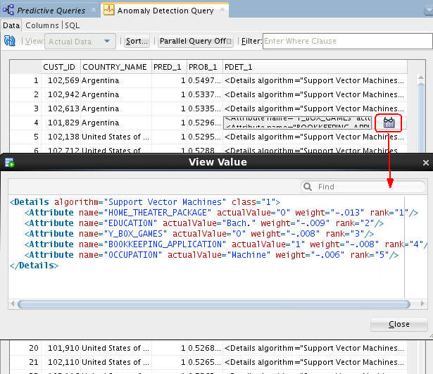
In the example, we select case number 4, with the Customer ID of 101,829. You can examine the prediction details if any case in the same way.
C. After you examine the prediction details, close the View Value window.
-
Close the Anomaly Detection Query tabbed window and Save the workflow by clicking the Save All icon in main toolbar.
Create and Execute a Feature Extraction Query
Feature Extraction models create new attributes (features) by using combinations of the original attribute. For example, you can group the demographic attributes for a set of customers into general characteristics that describe the customer.
When defining a Feature Extraction Query node, you specify similar attributes to a Feature Extraction model, but when the Query option is run, the Data Mining engine performs dynamic scoring of the clustering query without having to pre-define a model.
-
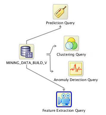
Add a Feature Extraction Query node to the workflow, as shown here:
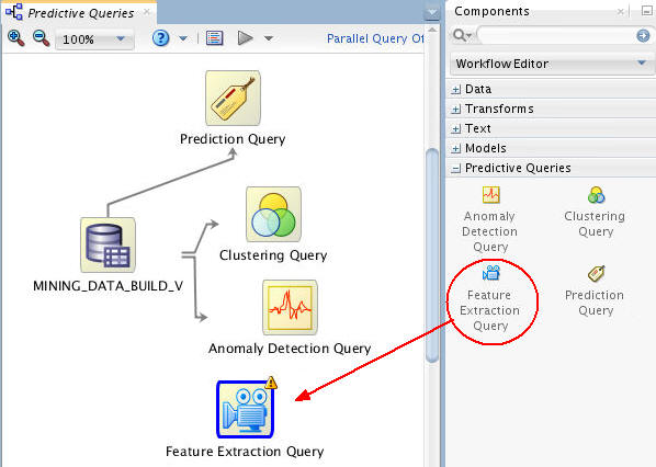
-
Connect the data source node to the Feature Extraction Query node like this:
A Feature Extraction Query node is defined by specifying the following:
- First, define the Case ID attribute.
- Second, specify the number of features to extract.
- Optionally, select one or more partition columns.
- Optionally, add or remove prediction output columns.
-
Double-click the Feature Extraction Query node to open the Edit Feature Extraction Query Node window. Then, perform the following on the Predictions tab:
A. Select CUST_ID as the Case ID attribute.
B. Accept the default value of 10 for number of clusters to compute.
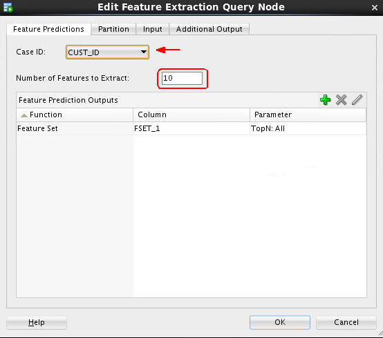
By default, only one Feature Prediction Output function is automatically defined: the Feature Set.
-
Next, select the Partition tab and perform the following:
A. Click the Add tool (green "+" icon).
B. Select the CUST_GENDER and EDUCATION attributes as partition columns.
C. Click OK.
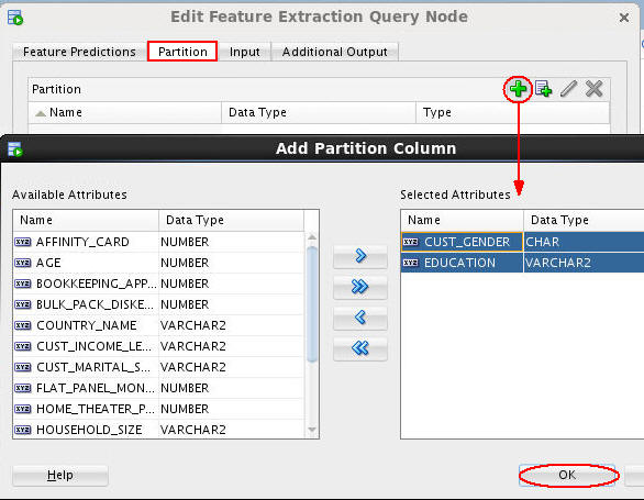
Note: This definition instructs the Data Mining server to build a unique virtual model for each distinct CUST_GENDER value and each distinct EDUCATION value.
-
Finally, click OK to close the Edit Feature Extraction Query Node window.
-
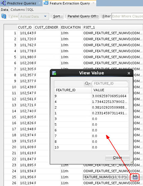
Right-click the Feature Extraction Query node and select View Data from the menu.
Result: A tabbed window displays the data, including the output columns and Feature Set definition column. Just like with the Anomaly Detection Query, expanded prediction details are also provided for Feature Extraction Query, as shown here:
-
Close the Feature Extraction Query tabbed window and Save the workflow by clicking the Save All icon in main toolbar.