HeatWave MySQL Performance

Performance comparison of MySQL HeatWave on OCI with Snowflake, Amazon Redshift, Amazon Aurora, and Amazon RDS for MySQL

Several performance comparisons have been run and the results are presented below. They focus on two different aspects.

• Query processing
  The performance comparison encompasses a variety of benchmarks—TPC-H, TPC-DS, and CH-benCHmark with different data set sizes (4 TB and 10 TB) to validate the speedup provided by MySQL HeatWave.
• Machine learning
  The performance experiments use a wide variety of publicly known data sets for machine learning classification and regression problems.

1. Common setup for analytic (OLAP) workload test for TPC-H and TPC-DS

• The workload is derived from the TPC’s TPC-H and TPC-DS benchmarks.*
• Generate data using the corresponding data generation tool.
• Provision and configure the target service.
• Create the corresponding schema on the target service instance.
• Import the data generated to the target service instance.
• Run queries derived from TPC-H or TPC-DS to test the performance.
• For best performance numbers, always do multiple runs of the query and ignore the first (cold) run.
• You can always do an explain plan to make sure you get the best expected plan.

2. Common setup for mixed workload test

• The workload is derived from CH-benCHmark.**
• The OLTPBench framework (with changes made to support MySQL HeatWave) was used to run the mixed workload benchmark.
• Provision and configure the target service instance.
• Create the mixed workload schema (TPC-C and CH-benCH) on the target service instance.
• Generate and load the 1,000 warehouse (100 GB) data set to the target service instance.
• Set the incoming rate of TPC-C transactions at 500 per second (30K transactions per minute) and the incoming rate of CH-benCH transactions at 4 per second (240 transactions per minute).
• Run 128 concurrent sessions of TPC-C (OLTP) and 4 concurrent sessions of CH-benCH (OLAP).
• Note the OLTP and OLAP throughput and average latency as reported.

3. MySQL HeatWave specific setup

• Optimal encodings are used for certain columns that will be loaded into MySQL HeatWave.
• Custom data placement is used for certain tables that will be loaded into MySQL HeatWave.
• Mark the tables as offloadable and load them into MySQL HeatWave.
• For each query, force offload to MySQL HeatWave using the hint (set_var(use_secondary_engine=forced)).
• A straight_join hint is required for certain queries to get the optimal query plan for MySQL HeatWave.
• For a detailed setup, reference the following:
  • MySQL HeatWave TPC-H GitHub for TPC-H.
  • MySQL HeatWave GitHub for TPC-DS and CH-benCHmark.

4. Snowflake on AWS specific setup

• For TPC-H, use clustering on ORDERS(o_orderdate) and LINEITEM(l_shipdate) tables.
• You can also try without clustering and pick the scheme that gives better performance.

5. Amazon Redshift specific setup

• Determine the best shape and cluster size for the experiments. In our experiments, we used ra3.4xlarge instance shape.
• For efficient data ingestion, follow the guidelines for enhanced VPC routing.
• Use the default parameters as specified by the Amazon documentation.
• Make sure the sort keys and distribution keys for each table are optimal for queries. The scripts provided by awslabs can be used for reference.

6. Amazon Aurora specific setup

• Use the largest shape possible so as much of the data can fit into the buffer cache as possible.
• For the 4 TB TPC-H data sets
  • Use the db.r5.24xlarge shapes.
  • Set the innodb_buffer_pool size to 630 GB.
  • Other settings that were modified from their default value in our TPC-H experiments are innodb_sort_buffer_size=67108864; lock_wait_timeout =86400; max_heap_table_size=103079215104; and tmp_table_size=103079215104.
• For the 1,000 warehouse TPC-C data set (used in mixed workload tests)
  • Use the db.r5.8xlarge shape.
  • Use the default parameter settings for innodb_buffer_pool and other parameters.
  • Disable the result cache.
  • Enable parallel query.
• Set aurora_disable_hash_join = 0 and aurora_parallel_query = ON to use parallel query.
• Follow the best practices for Aurora database configuration for any other tuning.
• For parallel query to work, make sure none of the tables are partitioned.
• A straight_join hint can be used if the query plan looks suboptimal.

7. Amazon RDS for MySQL specific setup

• Use the largest shape possible so as much of the data can fit into the buffer cache as possible.
• For the 4 TB TPC-H data sets, use the db.r5.24xlarge shape.
• Set the innodb_buffer_pool size to 650 GB.
• Other settings that were modified from their default value in our TPC-H experiments are innodb_buffer_pool_instances=64; innodb_page_cleaners=64; innodb_read_io_threads=64; temptable_max_ram=64424509440; max_heap_table_size=103079215104; and tmp_table_size=103079215104.
• Follow the best practices for Amazon RDS for any other tuning.
• Make sure all the primary and foreign key indexes are created.
• A straight_join hint can be used if the query plan looks suboptimal.

8. Results

Notes:

1. All costs include only the cost of compute. Storage costs aren’t included and are extra.
2. Redshift pricing is based on one-year reserved instance pricing (paid all upfront).
3. Snowflake pricing is based on standard edition on-demand pricing.
4. Google BigQuery pricing is based on annual flat-rate commitment (per 100 slots).
5. Azure Synapse pricing is based on the one-year reserved instance.

TPC-H results

4 TB TPC-H

	MySQL HeatWave	Snowflake on AWS	Amazon Redshift	Google BigQuery	Azure Synapse	Amazon Aurora	Amazon RDS for MySQL
Instance shape	HeatWave.512GB	-	ra3.4xlarge	-	DW 1,500c	db.r5.24xlarge	db.r5.24xlarge
Cluster size	4 + 1 MySQL.32	Medium (4)	2	400 slots	-	1	1
Geomean time	10.9 seconds	107.3 seconds	130.6 seconds	109.5 seconds	31.8 seconds
Total elapsed time	339 seconds	3,183 seconds	4,189 seconds	4,328 seconds	1,421 seconds	130 hours	338 hours
Annual cost	US$22,594	US$70,080	US$37,696	US$81,600	US$99,345	US$67,843	US$54,393

Note: Amazon Redshift, Snowflake, Azure Synapse, and Google BigQuery numbers for 4 TB TPC-H were provided by a third party in March 2022.

10 TB TPC-H

	MySQL HeatWave	Snowflake on AWS	Amazon Redshift	Google BigQuery	Databricks
Instance shape	HeatWave.512GB	-	ra3.4xlarge	-	-
Cluster size	10 + 1 MySQL.32	X-Large (16)	10	800 slots	Large
Geomean time	12.9	47.2	59.4	79.9	105.7
Total elapsed time	431 seconds	1,800 seconds	1,735 seconds	4,081 seconds	4,604 seconds
Annual cost	US$41,095	US$280,320	US$188,480	US$163,200	US$276,203

Note: Amazon Redshift, Snowflake, Google BigQuery, and Databricks numbers for 10 TB TPC-H were provided by a third party in May 2023.

^* Disclaimer: Benchmark queries are derived from the TPC-H benchmark, but results aren’t comparable to published TPC-H benchmark results since these don’t comply with the TPC-H specification.

TPC-DS results

10 TB TPC-DS

	MySQL HeatWave	Snowflake on AWS	Amazon Redshift	Google BigQuery	Azure Synapse
Instance shape	HeatWave.512GB	-	ra3.4xlarge	-	-
Cluster size	12 + 1 MySQL.32	X-Large (16)	8	800 slots	DW 2,500c
Geomean time	5 seconds	13 seconds	8 seconds	20.2 seconds	22.9 seconds
Total elapsed time	3,301 seconds	3,377 seconds	4,205 seconds	5,699 seconds	16,036 seconds
Annual cost	US$47,262	US$280,320	US$150,784	US$163,200	US$165,575

Note: The numbers for Amazon Redshift, Snowflake, Google BigQuery, and Azure Synapse for this 10 TB TPC-DS benchmark were provided by a third party in March 2022.

^* Disclaimer: Benchmark queries are derived from the TPC-DS benchmark, but results aren’t comparable to published TPC-DS benchmark results since these don’t comply with the TPC-DS specification.

Mixed benchmark results

1,000 warehouse (100 GB) CH-benCHmark

	MySQL HeatWave	Amazon Aurora
Instance shape	HeatWave.512GB	db.r5.8xlarge
Cluster size	2 + 1 MySQL.32	1
OLTP throughput (transactions per minute)	30,000	30,000
OLTP latency	0.02 seconds	0.02 seconds
OLAP throughput (transactions per minute)	6.6	0.06
OLAP latency	35 seconds	637 seconds
Annual cost	US$16,427	US$22,614

^** Disclaimer: CH-benCHmark queries are derived from the TPC-C and CH-benCH queries specified in the OLTPBench framework and aren’t comparable to any published TPC-C or CH-benCHmark results since these don’t comply with the TPC specifications.

Performance comparison of HeatWave AutoML with Redshift ML

Below is a setup for the comparison of two different ML problems: classification and regression. For a detailed setup, reference the HeatWave AutoML code for performance benchmarks on GitHub.

1. Common setup

• Datasets listed below are publicly available. Select a dataset to start your test.

  Datasets for classification

  Dataset	Explanation	Rows (training set)	Features
  Airlines	Predict flight delays.	377,568	8
  Bank Marketing	Direct marketing—banking products.	31,648	17
  CNAE-9	Documents with free text business descriptions of Brazilian companies.	757	857
  Connect-4	8-ply positions in the game of connect-4, in which neither player has won yet—predict win/loss.	47,290	43
  Fashion MNIST	Clothing classification problem.	60,000	785
  Nomao	Active learning is used to efficiently detect data that refers to the same place, based on the Nomao browser.	24,126	119
  Numerai	Data is cleaned, regularized, and encrypted global equity data.	67,425	22
  Higgs	Monte Carlo simulations.	10,500,000	29
  Census	Determine if a person’s income exceeds $50,000 a year.	32,561	15
  Titanic	Survival status of individuals.	917	14
  Credit Card Fraud	Identify fraudulent transactions.	199,364	30
  KDD Cup (appetency)	Predict the propensity of customers to buy new products.	35,000	230

  Datasets for regression

  Dataset	Explanation	Rows (training set)	Features
  Black Friday	Customer purchases on Black Friday.	116,774	10
  Diamonds	Predict the price of a diamond.	37,758	17
  Mercedes	Time the car took to pass testing.	2,946	377
  News Popularity	Predict the number of times articles were shared on social networks.	27,750	60
  NYC Taxi	Predict the tip amount for a New York City taxicab.	407,284	15
  Twitter	The popularity of a topic on social media.	408,275	78

• For each dataset, use 70% of the data for training and 30% of the data for testing. We recommend randomly selecting training data from the data set.
• Compute balanced accuracy for classification and R2 regression for regression on the test set.

2. HeatWave AutoML specific setup

• Use a HeatWave cluster with two HeatWave nodes.
• Run ML_TRAIN with the default arguments, and set task to classification or regression based on the dataset type.
• Score the generated model using ML_SCORE, with the metric set to balanced_accuracy for classification and R2 for regression.

3. Amazon Redshift ML specific setup

• Use a Redshift cluster with two nodes on ra3.4xlarge shape.
• Run CREATE_MODEL with the default values of MAX_CELLS (1M) and MAX_RUNTIME (5400s).
  • For the classification dataset, don't specify problem_type and let SageMaker detect the problem type.
  • For the regression dataset, run CREATE_MODEL with PROBLEM_TYPE being REGRESSION.
• Create custom SQL scoring functions to calculate balanced accuracy for classification and R2 for regression.

4. Setup for scalability test

• Test with 2, 4, 8, and 16 HeatWave node cluster.
• Run ML_TRAIN on all datasets described in the common setup section.
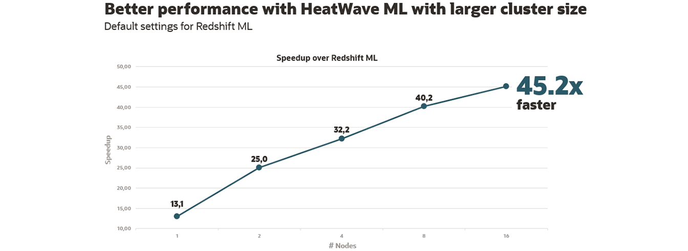
• Compute HeatWave AutoML versus Redshift ML speedup for training on every dataset via the following:
  • (Redshift ML default training time budget (90 minutes)) / (HeatWave AutoML end-to-end ML_TRAIN time)
• Compute the geometric mean of speedup across the datasets for each of the cluster configurations.
• Once all five geometric mean speedup values are obtained, plot the geomean speedup (y-axis) versus the cluster size (x-axis).

5. Results

Classification—performance comparison

Dataset	Accuracy		Training time (minutes)		Speedup
	Redshift ML	HeatWave AutoML	Redshift ML	HeatWave AutoML
Airlines	0.5	0.6524	90.00	2.71	33.21
Bank	0.8378	0.7115	90.00	3.72	24.19
CNAE-9	X	0.9167	X	5.91	X
Connect-4	0.6752	0.6970	90.00	7.13	12.62
Fashion MNIST	X	0.9073	X	181.85	X
Nomao	0.9512	0.9602	90.00	3.30	27.27
Numerai	0.5	0.5184	90.00	0.34	264.71
Higgs	0.5	0.758	90.00	68.58	1.31
Census	0.7985	0.7946	90.00	1.22	73.77
Titanic	0.9571	0.7660	90.00	0.47	191.49
CC Fraud	0.9154	0.9256	90.00	29.06	3.10
KDD Cup	X	0.5	X	3.55	X
Geomean	0.712	0.754	90.00	3.561	25.271

Classification—cost comparison

Dataset	Training cost ($)			Speedup
	Redshift ML list	Redshift ML with one-year plan	HeatWave AutoML
Airlines	20.00	6.23	0.0479	130.03
Bank	10.76	5.68	0.0658	86.30
CNAE-9	12.97	X	0.10458	X
Connect-4	20.00	6.18	0.1261	49.05
Fashion MNIST	20.00	X	3.2151	X
Nomao	20.00	5.96	0.0583	102.14
Numerai	20.00	5.49	0.0060	913.49
Higgs	20.00	7.27	1.2125	5.99
Census	9.77	6.12	0.0216	283.95
Titanic	0.26	5.60	0.0083	674.32
CC Fraud	20.00	6.70	0.0083	13.03
KDD Cup	20.00	X	0.5138	X
Geomean	10.62	6.115	0.063	97.13

Regression—performance comparison

Dataset	Accuracy		Training time (minutes)		Speedup
	Redshift ML	HeatWave AutoML	Redshift ML	HeatWave AutoML
Black Friday	0.54	0.53	90.00	1.14	78.80
Diamonds	0.98	0.98	90.00	2.40	37.42
Mercedes	X	0.61	X	1.16	X
News Popularity	0.02	0.01	90.00	0.60	149.13
NYC Taxi	0.19	0.25	90.00	7.34	12.26
Twitter	0.88	0.93	90.00	44.24	2.03
Geomean	0.27	0.26	90.00	3.52	25.58

Regression—cost comparison

Dataset	Training cost ($)			Lower cost
	Redshift ML list	Redshift ML cost with one-year plan	HeatWave AutoML	Scalability
Black Friday	20.00	2.95	0.02	146.10
Diamonds	7.55	5.13	0.04	120.61
Mercedes	20.00	X	0.02	X
News Popularity	20.00	4.15	0.01	389.08
NYC Taxi	20.00	2.82	0.13	21.76
Twitter	20.00	3.64	0.78	4.66
Geomean	17.00	3.64	0.06	58.66

Performance comparison of MySQL HeatWave on OCI with Snowflake, Amazon Redshift, Amazon Aurora, and Amazon RDS for MySQL

Several performance comparisons have been run and the results are presented below. They focus on two different aspects.

• Query processing
  The performance comparison encompasses a variety of benchmarks—TPC-H, TPC-DS, and CH-benCHmark with different data set sizes (4 TB and 10 TB) to validate the speedup provided by HeatWave.
• Machine learning
  The performance experiments use a wide variety of publicly known data sets for machine learning classification and regression problems.

1. Common setup for analytic (OLAP) workload test for TPC-H and TPC-DS

• The workload is derived from the TPC’s TPC-H and TPC-DS benchmarks.*
• Generate data using the corresponding data generation tool.
• Provision and configure the target service.
• Create the corresponding schema on the target service instance.
• Import the data generated to the target service instance.
• Run queries derived from TPC-H or TPC-DS to test the performance.
• For best performance numbers, always do multiple runs of the query and ignore the first (cold) run.
• You can always do an explain plan to make sure that you get the best expected plan.

2. Common setup for mixed workload test

• The workload is derived from CH-benCHmark.**
• The OLTPBench framework (with changes made to support HeatWave) was used to run the mixed workload benchmark.
• Provision and configure the target service instance.
• Create the mixed workload schema (TPC-C and CH-benCH) on the target service instance.
• Generate and load the 1,000 warehouse (100 GB) data set to the target service instance.
• Set incoming rate of TPC-C transactions at 500 per second (30K transactions per minute) and incoming rate of CH-benCH transactions at 4 per second (240 transactions per minute).
• Run 128 concurrent sessions of TPC-C (OLTP) and 4 concurrent sessions of CH-benCH (OLAP).
• Note the OLTP and OLAP throughput and average latency as reported.

3. HeatWave specific setup

• Optimal encodings are used for certain columns that will be loaded into HeatWave.
• Custom data placement is used for certain tables that will be loaded into HeatWave.
• Mark the tables as offloadable and load them into HeatWave.
• For each query, force offload to HeatWave using the hint (set_var(use_secondary_engine=forced)).
• A straight_join hint is required for certain queries to get the optimal query plan for HeatWave.
• For detailed setup, reference the following:
  • HeatWave TPC-H GitHub for TPC-H.
  • HeatWave GitHub for TPC-DS and CH-benCHmark.

4. Snowflake on AWS specific setup

• For TPC-H, use clustering on ORDERS(o_orderdate) and LINEITEM(l_shipdate) tables.
• You can also try without clustering and pick the scheme that gives better performance.

5. Amazon Redshift specific setup

• Determine the best shape and cluster size for the experiments. In our experiments, we used ra3.4xlarge instance shape.
• For efficient data ingestion, follow the guidelines for enhanced VPC routing.
• Use the default parameters as specified by the Amazon documentation.
• Make sure that the sort keys and distribution keys for each table are optimal for queries. The scripts provided by awslabs can be used for reference.

6. Amazon Aurora specific setup

• Use the largest shape possible so that as much of the data can fit into the buffer cache as possible.
• For the 4 TB TPC-H data sets
  • Use the db.r5.24xlarge shapes.
  • Set the innodb_buffer_pool size to 630 GB.
  • Here are other settings that were modified from their default value in our TPC-H experiments: innodb_sort_buffer_size=67108864; lock_wait_timeout =86400; max_heap_table_size=103079215104; tmp_table_size=103079215104.
• For the 1,000 warehouse TPC-C data set (used in mixed workload tests)
  • Use the db.r5.8xlarge shape.
  • Use the default parameter settings for innodb_buffer_pool and other parameters.
  • Disable result cache.
  • Enable parallel query.
• Set aurora_disable_hash_join = 0 and aurora_parallel_query = ON to use parallel query.
• Follow the best practices for Aurora database configuration for any other tuning.
• For parallel query to work, make sure that none of the tables are partitioned.
• A straight_join hint can be used if the query plan looks suboptimal.

7. Amazon RDS for MySQL specific setup

• Use the largest shape possible so that as much of the data can fit into the buffer cache as possible.
• For the 4 TB TPC-H data sets, use the db.r5.24xlarge shape.
• Set the innodb_buffer_pool size to 650 GB.
• Here are other settings that were modified from their default value in our TPC-H experiments: innodb_buffer_pool_instances=64; innodb_page_cleaners=64; innodb_read_io_threads=64; temptable_max_ram=64424509440; max_heap_table_size=103079215104; tmp_table_size=103079215104.
• Follow the best practices for Amazon RDS for any other tuning.
• Make sure all the primary and foreign key indexes are created.
• A straight_join hint can be used if the query plan looks suboptimal.

8. Results

Notes:

1. All costs include only the cost of compute. Storage costs aren’t included and are extra.
2. Redshift pricing is based on one-year reserved instance pricing (paid all upfront).
3. Snowflake pricing is based on standard edition on-demand pricing.
4. Google BigQuery pricing is based on annual flat-rate commitment (per 100 slots).
5. Azure Synapse pricing is based on the one-year reserved instance.

TPC-H results

4 TB TPC-H

	MySQL HeatWave	Snowflake on AWS	Amazon Redshift	Google BigQuery	Azure Synapse	Amazon Aurora	Amazon RDS for MySQL
Instance shape	HeatWave.512GB	-	ra3.4xlarge	-	DW 1,500c	db.r5.24xlarge	db.r5.24xlarge
Cluster size	4 + 1 MySQL.32	Medium (4)	2	400 slots	-	1	1
Geomean time	10.9 seconds	107.3 seconds	130.6 seconds	109.5 seconds	31.8 seconds
Total elapsed time	339 seconds	3,183 seconds	4,189 seconds	4,328 seconds	1,421 seconds	130 hours	338 hours
Annual cost	US$22,594	US$70,080	US$37,696	US$81,600	US$99,345	US$67,843	US$54,393

Note: Amazon Redshift, Snowflake, Azure Synapse, and Google BigQuery numbers for 4 TB TPC-H were provided by a third party in March 2022.

10 TB TPC-H

	MySQL HeatWave	Snowflake on AWS	Amazon Redshift	Google BigQuery	Databricks
Instance shape	HeatWave.512GB	-	ra3.4xlarge	-	-
Cluster size	10 + 1 MySQL.32	X-Large (16)	10	800 slots	Large
Geomean time	12.9	47.2	59.4	79.9	105.7
Total elapsed time	431 seconds	1,800 seconds	1,735 seconds	4,081 seconds	4,604 seconds
Annual cost	US$41,095	US$280,320	US$188,480	US$163,200	US$276,203

Note: Amazon Redshift, Snowflake, Google BigQuery, and Databricks numbers for 10 TB TPC-H were provided by a third party in May 2023.

^* Disclaimer: Benchmark queries are derived from the TPC-H benchmark, but results aren’t comparable to published TPC-H benchmark results since these don’t comply with the TPC-H specification.

TPC-DS results

10 TB TPC-DS

	MySQL HeatWave	Snowflake on AWS	Amazon Redshift	Google BigQuery	Azure Synapse
Instance shape	HeatWave.512GB	-	ra3.4xlarge	-	-
Cluster size	12 + 1 MySQL.32	X-Large (16)	8	800 slots	DW 2,500c
Geomean time	5 seconds	13 seconds	8 seconds	20.2 seconds	22.9 seconds
Total elapsed time	3,301 seconds	3,377 seconds	4,205 seconds	5,699 seconds	16,036 seconds
Annual cost	US$47,262	US$280,320	US$150,784	US$163,200	US$165,575

Note: The numbers for Amazon Redshift, Snowflake, Google BigQuery, and Azure Synapse for this 10 TB TPC-DS benchmark were provided by a third party in March 2022.

^* Disclaimer: Benchmark queries are derived from the TPC-DS benchmark, but results aren’t comparable to published TPC-DS benchmark results since these don’t comply with the TPC-DS specification.

Mixed benchmark results

1,000 warehouse (100 GB) CH-benCHmark

	MySQL HeatWave	Amazon Aurora
Instance shape	HeatWave.512GB	db.r5.8xlarge
Cluster size	2 + 1 MySQL.32	1
OLTP throughput (transactions per minute)	30,000	30,000
OLTP latency	0.02 seconds	0.02 seconds
OLAP throughput (transactions per minute)	6.6	0.06
OLAP latency	35 seconds	637 seconds
Annual cost	US$16,427	US$22,614

^** Disclaimer: CH-benCHmark queries are derived from the TPC-C and CH-benCH queries specified in the OLTPBench framework and aren’t comparable to any published TPC-C or CH-benCHmark results since these don’t comply with the TPC specifications.

Performance comparison of HeatWave AutoML with Redshift ML

Setup for the comparison of two different ML problems: classification and regression. For detailed setup, reference the HeatWave AutoML code for performance benchmarks on GitHub.

1. Common setup

• Datasets listed below are publicly available. Select a dataset to start your test.

  Datasets for classification

  Dataset	Explanation	Rows (Training set)	Features
  Airlines	Predict flight delays.	377,568	8
  Bank Marketing	Direct marketing—banking products.	31,648	17
  CNAE-9	Documents with free text business descriptions of Brazilian companies.	757	857
  Connect-4	8-ply positions in the game of connect-4, in which neither player has won yet—predict win/loss.	47,290	43
  Fashion MNIST	Clothing classification problem.	60,000	785
  Nomao	Active learning is used to efficiently detect data that refers to the same place, based on the Nomao browser.	24,126	119
  Numerai	Data is cleaned, regularized, and encrypted global equity data.	67,425	22
  Higgs	Monte Carlo simulations.	10,500,000	29
  Census	Determine if a person’s income exceeds $50,000 a year.	32,561	15
  Titanic	Survival status of individuals.	917	14
  Credit Card Fraud	Identify fraudulent transactions.	199,364	30
  KDD Cup (appetency)	Predict the propensity of customers to buy new products.	35,000	230

  Datasets for regression

  Dataset	Explanation	Rows (Training set)	Features
  Black Friday	Customer purchases on Black Friday.	116,774	10
  Diamonds	Predict the price of a diamond.	37,758	17
  Mercedes	Time the car took to pass testing.	2,946	377
  News Popularity	Predict the number of times articles were shared on social networks.	27,750	60
  NYC Taxi	Predict the tip amount for a New York City taxicab.	407,284	15
  Twitter	The popularity of a topic on social media.	408,275	78

• For each dataset, use 70% of the data for training and 30% of the data for testing. We recommend randomly selecting training data from the data set.
• Compute balanced accuracy for classification and R2 regression for regression on the test set.

2. HeatWave AutoML specific setup

• Use a HeatWave cluster with two HeatWave nodes.
• Run ML_TRAIN with the default arguments, and set task to classification or regression based on the dataset type.
• Score the generated model using ML_SCORE, with the metric set to balanced_accuracy for classification and R2 for regression.

3. Amazon Redshift ML specific setup

• Use a Redshift cluster with two nodes on ra3.4xlarge shape.
• Run CREATE_MODEL with the default values of MAX_CELLS (1M) and MAX_RUNTIME (5400s).
  • For classification dataset, do not specify problem_type and let SageMaker detect the problem type.
  • For regression dataset, run CREATE_MODEL with PROBLEM_TYPE being REGRESSION.
• Create custom SQL scoring functions to calculate balanced accuracy for classification and R2 for regression.

4. Setup for scalability test

• Test with 2, 4, 8, and 16 HeatWave node cluster.
• Run ML_TRAIN on all datasets described in common setup section.
• Compute HeatWave AutoML versus Redshift ML speedup for training on every dataset via the following:
  • (Redshift ML default training time budget (90 minutes)) / (HeatWave AutoML end-to-end ML_TRAIN time)
• Compute geometric mean of speedup across the datasets for each of the cluster configurations.
• Once all five geometric mean speedup values are obtained, plot geomean speedup (y-axis) versus cluster size (x-axis).

5. Results

Classification—Performance Comparison

Dataset	Accuracy		Training time (minutes)		Speedup
	Redshift ML	HeatWave AutoML	Redshift ML	HeatWave AutoML
Airlines	0.5	0.6524	90.00	2.71	33.21
Bank	0.8378	0.7115	90.00	3.72	24.19
CNAE-9	X	0.9167	X	5.91	X
Connect-4	0.6752	0.6970	90.00	7.13	12.62
Fashion MNIST	X	0.9073	X	181.85	X
Nomao	0.9512	0.9602	90.00	3.30	27.27
Numerai	0.5	0.5184	90.00	0.34	264.71
Higgs	0.5	0.758	90.00	68.58	1.31
Census	0.7985	0.7946	90.00	1.22	73.77
Titanic	0.9571	0.7660	90.00	0.47	191.49
CC Fraud	0.9154	0.9256	90.00	29.06	3.10
KDD Cup	X	0.5	X	3.55	X
Geomean	0.712	0.754	90.00	3.561	25.271

Classification—Cost Comparison

Dataset	Training cost ($)			Speedup
	Redshift ML list	Redshift ML with one-year plan	HeatWave AutoML
Airlines	20.00	6.23	0.0479	130.03
Bank	10.76	5.68	0.0658	86.30
CNAE-9	12.97	X	0.10458	X
Connect-4	20.00	6.18	0.1261	49.05
Fashion MNIST	20.00	X	3.2151	X
Nomao	20.00	5.96	0.0583	102.14
Numerai	20.00	5.49	0.0060	913.49
Higgs	20.00	7.27	1.2125	5.99
Census	9.77	6.12	0.0216	283.95
Titanic	0.26	5.60	0.0083	674.32
CC Fraud	20.00	6.70	0.0083	13.03
KDD Cup	20.00	X	0.5138	X
Geomean	10.62	6.115	0.063	97.13

Regression—Performance Comparison

Dataset	Accuracy		Training time (minutes)		Speedup
	Redshift ML	HeatWave AutoML	Redshift ML	HeatWave AutoML
Black Friday	0.54	0.53	90.00	1.14	78.80
Diamonds	0.98	0.98	90.00	2.40	37.42
Mercedes	X	0.61	X	1.16	X
News Popularity	0.02	0.01	90.00	0.60	149.13
NYC Taxi	0.19	0.25	90.00	7.34	12.26
Twitter	0.88	0.93	90.00	44.24	2.03
Geomean	0.27	0.26	90.00	3.52	25.58

Regression—Cost Comparison

Dataset	Training cost ($)			Lower cost
	Redshift ML list	Redshift ML cost with one-year plan	HeatWave AutoML	Scalability
Black Friday	20.00	2.95	0.02	146.10
Diamonds	7.55	5.13	0.04	120.61
Mercedes	20.00	X	0.02	X
News Popularity	20.00	4.15	0.01	389.08
NYC Taxi	20.00	2.82	0.13	21.76
Twitter	20.00	3.64	0.78	4.66
Geomean	17.00	3.64	0.06	58.66

Performance comparison of MySQL HeatWave on AWS with Amazon Aurora, Amazon Redshift, Snowflake, Azure Synapse Analytics, and Google BigQuery

Several performance comparisons have been run and the results are presented below. They focus on two different aspects.

• OLAP performance
  The performance comparison includes the TPC-H benchmark* with a dataset of 4 TB, to validate the speedup provided by MySQL HeatWave on AWS.
• OLTP performance
  The performance comparison includes the TPC-C benchmark** with a dataset of 10 GB to validate the throughput provided by MySQL HeatWave on AWS.

1. Common setup for analytic (OLAP) workload test for TPC-H

• The workload is derived from TPC's TPC-H benchmarks.*
• Generate data using the corresponding data generation tool.
• Provision and configure the target service.
• Create the corresponding schema on the target service instance.
• Import the data generated to the target service instance.
• Run queries derived from TPC-H to test the performance.
• For best performance numbers, always do multiple runs of the query and ignore the first (cold) run.
• You can always do an explain plan to make sure you get the best expected plan.

2. Common setup for transactional (OLTP) workload test for TPC-C

• The workload is derived from the TPC-C benchmark.**
• The sysbench framework (with additional Lua scripts for TPC-C) is used to run the TPC-C benchmark.
• Provision and configure the target service instance.
• Create the OLTP workload schema (TPC-C) on the target service instance.
• Generate and load the 100 W (10 GB) dataset to the target service instance.
• Start with one concurrent session and gradually increase the number of concurrent sessions to see the impact on throughput and latency.
• Note the OLTP throughput as reported.

3. HeatWave specific setup

• The MySQL.32.256GB shape is used for the MySQL node and the HeatWave.256GB shape is used for the HeatWave nodes.
• For TPC-H benchmark
  • Optimal encodings are used for certain columns that will be loaded into HeatWave.
  • Custom data placement is used for certain tables that will be loaded into HeatWave.
  • Mark the tables as offloadable and load them into HeatWave.
  • For each query, force offload to HeatWave using the hint (set_var(use_secondary_engine=forced)).
  • A straight_join hint is required for certain queries to get the optimal query plan for HeatWave.
• For TPC-C benchmark
  • Make sure the client and HeatWave instance are in the same physical AZ.
• For a detailed setup, reference the following:
  • HeatWave TPC-H GitHub for TPC-H.
  • HeatWave GitHub for TPC-C benchmark.

4. Snowflake on AWS specific setup

• In the experiments, a medium-size cluster is used.
• For TPC-H, use clustering on ORDERS(o_orderdate) and LINEITEM(l_shipdate) tables.
• You can also try without clustering and pick the scheme that gives better performance.

5. Amazon Redshift specific setup

• Determine the best shape and cluster size for the experiments. In the experiments, two nodes of ra3.4xlarge instance shape were used.
• For efficient data ingestion, follow the guidelines for enhanced VPC routing.
• Use the default parameters as specified by the Amazon documentation.
• Make sure the sort keys and distribution keys for each table are optimal for queries. The scripts provided by awslabs can be used for reference.

6. Microsoft Azure Synapse specific setup

• In the experiments, DW 1500c cluster is used.

7. Google BigQuery specific setup

• In the experiments, 400 slots are used for running the queries.

8. Amazon Aurora specific setup for TPC-C benchmark

• Use the db.r5.8xlarge shape.
• Use the default parameter settings for innodb_buffer_pool and other parameters.
• Set adaptive hash index = off; replication = off; redo_log = off.
• Follow the best practices for Aurora database configuration for any other tuning.

9. Results

4 TB TPC-H (September 2022)

	MySQL HeatWave on AWS	Amazon Redshift	Snowflake on AWS	Azure Synapse	Google BigQuery
Instance shape	HeatWave.256GB + MySQL.32.256GB	ra3.4xlarge	-	-	-
Cluster size	10 + 1 MySQL node	2 nodes	Medium	DW 1500c	400 slots
Geomean time	6.53 seconds	130.62 seconds	107.27 seconds	31.8 seconds	109.47 seconds
Price-performance	US$0,023	US$0,156	US$0,238	US$0,1	US$0,283

Note: Redshift, Snowflake, Synapse and Google BigQuery numbers for 4 TB TPC-H are provided by a third party.

Note: Redshift pricing is based on one-year reserved instance pricing (paid all upfront). Snowflake pricing is based on standard edition on-demand pricing. Google BigQuery pricing is based on annual flat-rate commitment (per 100 slots). Azure Synapse pricing is based on the one-year reserved instance.

*Disclaimer: Benchmark queries are derived from the TPC-H benchmarks, but results aren’t comparable to published TPC-H benchmark results since these don't comply with the TPC-H specifications.

100W (10 GB) TPC-C (September 2022)

MySQL HeatWave on AWS node type: MySQL.32.256GB.
Amazon Aurora node type: db.r5.8xlarge.

Concurrency	1	4	16	64	128	256	512	1,024	2,048	4,096
Amazon Aurora throughput	116	471	1,411	3,138	4,615	5,081	4,784	2,487	574	245
MySQL HeatWave throughput	86	322	1,040	3,314	5,198	6,192	6,195	5,953	6,080	6,001

Note: Aurora numbers for TPC-C are provided by a third party.

**Disclaimer: Benchmark queries are derived from the TPC-C benchmarks, but results aren’t comparable to published TPC-C benchmark results since these don’t comply with the TPC-C specifications.

Performance comparison of HeatWave Lakehouse with Snowflake, Amazon Redshift, Google BigQuery, and Databricks

Performance comparisons for a very large data set were run, and the results are presented below. The results focus on both load and query performance.

The content below details the setup for the TPC-H analytic workload for a scale factor of 500,000 (a data set size of 500 TB) and the TPC-DS analytic workload with a data set size of 100 TB.

1. Common setup for analytic workload test for TPC-H and TPC-DS

The workload is derived from the TPC's TPC-H and TPC-DS benchmarks.^*

• Generate data using the corresponding data generation tool.
• Keep the generated data in a bucket in the respective cloud service (Oracle Cloud Infrastructure, Amazon Web Services, or Google Cloud Platform). Ensure the bucket is in the same region where the database system will be provisioned.
• Provision and configure the target service.
• Create the corresponding schema on the target service instance.
• Load the data generated to the target service instance and measure the load time.
• Run queries derived from TPC-H or TPC-DS to test the performance.
• For best performance numbers, always do multiple runs of the query and ignore the first (cold) run.
• You can always run an explain plan to make sure you get the best expected plan.

2. HeatWave Lakehouse specific setup

• For TPC-H, a 512-node HeatWave cluster is used for the experiments.
• For TPC-DS, a 120-node HeatWave cluster is used for the experiments.
• Custom data placement is used for certain tables that will be loaded into HeatWave Lakehouse.
• Mark the tables as offloadable and load them into HeatWave.

• For a detailed setup, reference the following:

  • HeatWave TPC-H GitHub for TPC-H
  • HeatWave TPC-DS GitHub for TPC-DS

3. Snowflake on AWS specific setup

• For TPC-H, use clustering on ORDERS(o_orderdate) and LINEITEM(l_shipdate) tables.
• You can also try without clustering and pick the scheme that gives better performance.

• Determine the best cluster size for the experiments.

  • For 500 TB TPC-H, a 4X-Large cluster is used.
  • For 100 TB TPC-DS, a 3X-Large cluster is used.

4. Amazon Redshift specific setup

• Determine the best shape and cluster size for the experiments.

  • For 500 TB TPC-H, 20 nodes of a ra3.16xlarge instance are used in these experiments.
  • For 100 TB TPC-DS, 10 nodes of a ra3.16xlarge instance are used.
• For efficient data ingestion, follow the guidelines for enhanced VPC routing.
• Use the default parameters as specified by the Amazon documentation.
• Make sure the sort keys and distribution keys for each table are optimal for queries.

5. Google BigQuery specific setup

• Determine the ideal number of slots for the experiments.

  • For 500 TB TPC-H, 6,400 slots are used.
  • For 100 TB TPC-DS, 3,200 slots are used.

6. Databricks on AWS specific setup

• Determine the ideal cluster size for the experiments.

  • For 500 TB TPC-H, a 3X-Large cluster is used.
  • For 100 TB TPC-DS, a 2X-Large cluster is used.

7. Results

Notes:

1. Redshift pricing is based on one-year reserved instance pricing (paid all upfront).
2. Snowflake pricing is based on standard edition on-demand pricing.
3. Google BigQuery pricing is based on annual flat-rate commitment (per 100 slots).
4. Databricks Enterprise Sql Pro pricing is based on one-year reserved EC2 instance.

500 TB TPC-H

	HeatWave Lakehouse	Snowflake on AWS	Amazon Redshift	Google BigQuery	Databricks on AWS
Instance shape	HeatWave.512GB	-	ra3.16xlarge	6,400 slots	-
Cluster size	512 + 1 MySQL.32	4X-Large (128)	20	-	3X-Large
Load time	4.43 hours	9.04 hours	40.86 hours	38.2 hours	25.42 hours
Geomean time	47 seconds	821 seconds	423.3 seconds	1,713 seconds	788.1 seconds
Total query time	2,150 seconds	39,040 seconds	32,715 seconds	76,180 seconds	37,729 seconds
Annual cost	US$1,709,022	US$2,300,160	US$1,544,268	US$1,446,900	US$1,822,817

100 TB TPC-DS—single user

	HeatWave Lakehouse	Snowflake on AWS	Amazon Redshift	Google BigQuery	Databricks on AWS
Instance shape	HeatWave.512GB	-	ra3.16xlarge	3,200 slots	-
Cluster size	120 + 1 MySQL.32	3X-Large (128)	10	-	2X-Large
Load time	1.21 hours	3.3 hours	7.74 hours	3.63 hours	7.46 hours
Geomean time	6.45 seconds	21.32 seconds	11.67 seconds	35.26 seconds	26.63 seconds
Total query time	3,719 seconds	5,379 seconds	5,108 seconds	11,694 seconds	13,704 seconds
Annual cost	US$404,282	US$1,132,781	US$761,173	US$681,408	US$913,563

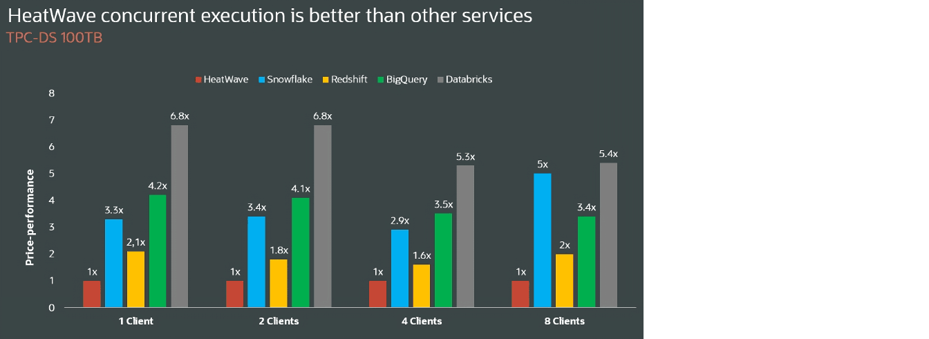
100 TB TPC-DS—concurrent users

HeatWave concurrent execution is better than other services

TPC-DS 100TB

	HeatWave	Snowflake	Redshift	BigQuery	Databricks
1 client price-performance	1X	3.3X	2.1X	4.2X	6.8X
2 clients price-performance	1X	3.4X	1.8X	4.1X	6.8X
4 clients price-performance	1X	2.9X	1.6X	3.5X	5.3X
8 clients price-performance	1X	5X	2X	3.4X	5.4X

Note: Snowflake, Redshift, Google BigQuery, and Databricks numbers for 500 TB TPC-H and 100 TB TPC-DS are provided by a third party.

^*Benchmark queries are derived from TPC-H and TPC-DS benchmarks, but results aren’t comparable to published TPC-H and TPC-DS benchmark results since these don’t comply with the TPC-H and TPC-DS specifications.

Performance comparisons of HeatWave GenAI with Snowflake, Databricks, and Google BigQuery

Performance comparisons for a variety of queries on data sets of different sizes were done, and the results are presented below.

The content below details the setup for three data sets: Wikipedia (1.7 GB), dbpedia (3 GB), and MIRACL (300 GB).

Common setup

Download the data sets required for the queries.

• Wikipedia
• dbpedia
• MIRACL_en
• MIRACL_de
• msmacro

Once the data is downloaded

1. Provision and configure the target service.
2. Create the corresponding schema on the target service instance.
3. Import the data to the target service instance.
4. Run the queries to test the performance.
5. The queries are a mix of queries that do nearest neighbor top 10 results (in ascending and descending order) with different distance metrics, do nearest neighbor queries with additional predicates, do joins between tables with different languages, do semantic searches on the joined result, use embedding column as an aggregation result, do distance-based filtering, and so forth.
6. For best performance numbers, always do multiple runs of the query and ignore the first (cold) run.

Results

Notes

1. All costs only include the compute cost. Storage costs aren’t included.
2. Snowflake pricing is based on standard edition on-demand pricing.
3. Google BigQuery pricing is based on standard edition pay-as-you-go pricing.
4. Databricks pricing is based on a premium SQL serverless compute 2X-small shape, plus the cost of Mosaic vector search.

Vector search results

	HeatWave GenAI	Snowflake	Databricks	Google BigQuery
Instance shape	HeatWave.512GB	-	-	100 slots
Cluster size	1 + 1 MySQL.32	X-Small	25units+2xLarge	-
Hourly cost	US$1.50	US$2.00	US$9.80	US$4.00
Total query time	16 seconds	466 seconds	238 seconds	288 seconds
HeatWave GenAI performance advantage	-	29X	15X	18X

Note: All numbers were provided by a third party in June 2024.

Performance comparisons of HeatWave Vector Store on AWS with Knowledge Bases for Amazon Bedrock

Performance comparisons for creating a vector store using a variety of documents were completed and the results are presented below.

Data set used
100K files from Wikipedia, converted into different formats.

Setup

1. Upload the documents into the Amazon S3 bucket.
2. Provision and configure HeatWave on AWS as well as Knowledge Bases for Amazon Bedrock.
3. Trigger vector store creation from the uploaded documents.

Results

Notes

1. All costs only include the compute cost. Storage costs aren’t included.
2. The vector store creation cost for HeatWave is based on the following configuration: one MySQL node with 2 vCPUs and 10 HeatWave cluster nodes.
3. The vector store creation for Knowledge Bases for Amazon Bedrock includes naming the knowledge base, configuring the data source in S3, using Cohere Embed English v3 for embedding, followed by “quick create of vector store.” The costs considered in the comparative measurements for embedding the ingested documents were recorded from the AWS bill and then discounted by 50% for batch discount.

	HeatWave (10 nodes)	Knowledge Bases for Amazon Bedrock
100K DOCX documents
Vector store creation time	0.54 hours	8.02 hours
Vector store creation cost	US$4.29	US$9.09
100K HTML documents
Vector store creation time	0.65 hours	8.07 hours
Vector store creation cost	US$5.12	US$9.61
100K PDF documents
Vector store creation time	0.38 hours	11.45 hours
Vector store creation cost	US$3.01	US$13.65
100K TXT documents
Vector store creation time	0.76 hours	18.86 hours
Vector store creation cost	US$5.99	US$31.42